MASH v FLASH GTEx analysis: “Top 20” v “Zero”
Last updated: 2018-08-05
workflowr checks: (Click a bullet for more information)-
✔ R Markdown file: up-to-date
Great! Since the R Markdown file has been committed to the Git repository, you know the exact version of the code that produced these results.
-
✔ Environment: empty
Great job! The global environment was empty. Objects defined in the global environment can affect the analysis in your R Markdown file in unknown ways. For reproduciblity it’s best to always run the code in an empty environment.
-
✔ Seed:
set.seed(20180609)The command
set.seed(20180609)was run prior to running the code in the R Markdown file. Setting a seed ensures that any results that rely on randomness, e.g. subsampling or permutations, are reproducible. -
✔ Session information: recorded
Great job! Recording the operating system, R version, and package versions is critical for reproducibility.
-
Great! You are using Git for version control. Tracking code development and connecting the code version to the results is critical for reproducibility. The version displayed above was the version of the Git repository at the time these results were generated.✔ Repository version: 3333b18
Note that you need to be careful to ensure that all relevant files for the analysis have been committed to Git prior to generating the results (you can usewflow_publishorwflow_git_commit). workflowr only checks the R Markdown file, but you know if there are other scripts or data files that it depends on. Below is the status of the Git repository when the results were generated:
Note that any generated files, e.g. HTML, png, CSS, etc., are not included in this status report because it is ok for generated content to have uncommitted changes.Ignored files: Ignored: .DS_Store Ignored: .Rhistory Ignored: .Rproj.user/ Ignored: data/ Ignored: docs/.DS_Store Ignored: docs/images/.DS_Store Ignored: docs/images/.Rapp.history Ignored: output/.DS_Store Ignored: output/.Rapp.history Ignored: output/MASHvFLASHgtex/.DS_Store Ignored: output/MASHvFLASHsims/.DS_Store Ignored: output/MASHvFLASHsims/backfit/.DS_Store Ignored: output/MASHvFLASHsims/backfit/.Rapp.history
Expand here to see past versions:
| File | Version | Author | Date | Message |
|---|---|---|---|---|
| Rmd | 3333b18 | Jason Willwerscheid | 2018-08-05 | wflow_publish(“analysis/Top20vZero.Rmd”) |
| html | 5ba9a9a | Jason Willwerscheid | 2018-08-05 | Build site. |
| html | 1d57c08 | Jason Willwerscheid | 2018-08-04 | Build site. |
| Rmd | c018ca3 | Jason Willwerscheid | 2018-08-04 | wflow_publish(c(“analysis/index.Rmd”, “analysis/Top20vZero.Rmd”)) |
Introduction
This analysis compares the “Top 20” FLASH fit to the “Zero” FLASH fit (which does not include any canonical loadings). See here for fitting details. See here and here for introductions to the plots. Because the first data-driven loading in the “Zero” fit generally acts as a surrogate for the “equal effects” loading in the “Top 20” fit, I combine the two loadings in the plots below for ease of interpretation.
library(mashr)Loading required package: ashrdevtools::load_all("/Users/willwerscheid/GitHub/flashr/")Loading flashrgtex <- readRDS(gzcon(url("https://github.com/stephenslab/gtexresults/blob/master/data/MatrixEQTLSumStats.Portable.Z.rds?raw=TRUE")))
strong <- t(gtex$strong.z)
fpath <- "./output/MASHvFLASHgtex2/"
top20_final <- readRDS(paste0(fpath, "top20.rds"))
zero_final <- readRDS(paste0(fpath, "zero.rds"))
all_fl_lfsr <- readRDS(paste0(fpath, "fllfsr.rds"))
top20_lfsr <- all_fl_lfsr[[4]]
zero_lfsr <- all_fl_lfsr[[5]]
top20_pm <- flash_get_fitted_values(top20_final)
zero_pm <- flash_get_fitted_values(zero_final)missing.tissues <- c(7, 8, 19, 20, 24, 25, 31, 34, 37)
gtex.colors <- read.table("https://github.com/stephenslab/gtexresults/blob/master/data/GTExColors.txt?raw=TRUE", sep = '\t', comment.char = '')[-missing.tissues, 2]
OHF.colors <- c("tan4", "tan3")
zero.colors <- c("black", gray.colors(19, 0.2, 0.9),
gray.colors(17, 0.95, 1))
plot_test <- function(n, lfsr, pm, method_name) {
plot(strong[, n], pch=1, col="black", xlab="", ylab="", cex=0.6,
ylim=c(min(c(strong[, n], 0)), max(c(strong[, n], 0))),
main=paste0("Test #", n, "; ", method_name))
size = rep(0.6, 44)
shape = rep(15, 44)
signif <- lfsr[, n] <= .05
shape[signif] <- 17
size[signif] <- 1.35 - 15 * lfsr[signif, n]
size <- pmin(size, 1.2)
points(pm[, n], pch=shape, col=as.character(gtex.colors), cex=size)
abline(0, 0)
}
plot_ohf_v_ohl_loadings <- function(n, ohf_fit, ohl_fit, ohl_name,
legend_pos = "bottomright") {
ohf <- abs(ohf_fit$EF[n, ] * apply(abs(ohf_fit$EL), 2, max))
ohl <- -abs(ohl_fit$EF[n, ] * apply(abs(ohl_fit$EL), 2, max))
data <- rbind(c(ohf, rep(0, length(ohl) - 45)),
c(ohl[1:45], rep(0, length(ohf) - 45),
ohl[46:length(ohl)]))
colors <- c("black",
as.character(gtex.colors),
OHF.colors,
zero.colors[1:(length(ohl) - 45)])
x <- barplot(data, beside=T, col=rep(colors, each=2),
main=paste0("Test #", n, " loadings"),
legend.text = c("OHF", ohl_name),
args.legend = list(x = legend_pos, bty = "n", pch="+-",
fill=NULL, border="white"))
text(x[2*(46:47) - 1], min(data) / 10,
labels=as.character(1:2), cex=0.4)
text(x[2*(48:ncol(data))], max(data) / 10,
labels=as.character(1:(length(ohl) - 45)), cex=0.4)
}
plot_ohl_v_zero_loadings <- function(n, ohl_fit, zero_fit, ohl_name,
legend_pos = "topright") {
ohl <- abs(ohl_fit$EF[n, ] * apply(abs(ohl_fit$EL), 2, max))
# Combine equal effects and first data-driven loading
ohl[1] <- ohl[1] + ohl[46]
ohl <- ohl[-46]
zero <- -abs(zero_fit$EF[n, ] * apply(abs(zero_fit$EL), 2, max))
data <- rbind(c(ohl, rep(0, length(zero) - length(ohl) + 44)),
c(zero[1], rep(0, 44), zero[2:length(zero)]))
colors <- c("black", as.character(gtex.colors), zero.colors)
x <- barplot(data, beside=T, col=rep(colors, each=2),
main=paste0("Test #", n, " loadings"),
legend.text = c(ohl_name, "Zero"),
args.legend = list(x = legend_pos, bty = "n", pch="+-",
fill=NULL, border="white"))
text(x[2*(seq(46, ncol(data), by=2)) - 1], min(data) / 10,
labels=as.character(seq(2, length(zero), by=2)), cex=0.4)
}
compare_methods <- function(lfsr1, lfsr2, pm1, pm2) {
res <- list()
res$first_not_second <- find_A_not_B(lfsr1, lfsr2)
res$lg_first_not_second <- find_large_A_not_B(lfsr1, lfsr2)
res$second_not_first <- find_A_not_B(lfsr2, lfsr1)
res$lg_second_not_first <- find_large_A_not_B(lfsr2, lfsr1)
res$diff_pms <- find_overall_pm_diff(pm1, pm2)
return(res)
}
# Find tests where many conditions are significant according to
# method A but not according to method B.
find_A_not_B <- function(lfsrA, lfsrB) {
select_tests(colSums(lfsrA <= 0.05 & lfsrB > 0.05))
}
# Find tests where many conditions are highly significant according to
# method A but are not significant according to method B.
find_large_A_not_B <- function(lfsrA, lfsrB) {
select_tests(colSums(lfsrA <= 0.01 & lfsrB > 0.05))
}
find_overall_pm_diff <- function(pmA, pmB, n = 4) {
pm_diff <- colSums((pmA - pmB)^2)
return(order(pm_diff, decreasing = TRUE)[1:4])
}
# Get at least four (or min_n) "top" tests.
select_tests <- function(colsums, min_n = 4) {
n <- 45
n_tests <- 0
while (n_tests < min_n && n > 0) {
n <- n - 1
n_tests <- sum(colsums >= n)
}
return(which(colsums >= n))
}plot_it <- function(n, legend.pos = "topright") {
par(mfrow=c(1, 2))
plot_test(n, top20_lfsr, top20_pm, "Top 20")
plot_test(n, zero_lfsr, zero_pm, "Zero")
par(mfrow=c(1, 1))
plot_ohl_v_zero_loadings(n, top20_final, zero_final, "Top 20",
legend.pos)
}Significant for Top 20, not Zero
It is possible to distinguish three classes of cases where the “Top 20” method picks out significant effects but the “Zero” method does not. I give a typical example for each class.
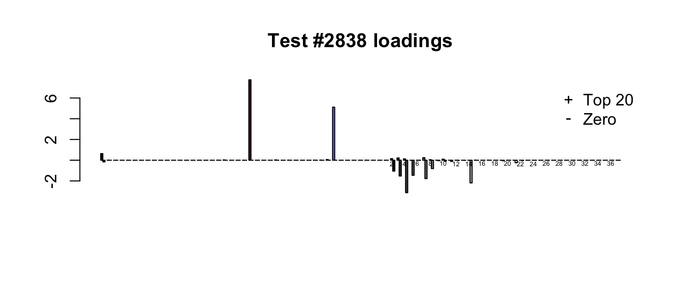
- Because the “Zero” fit does not include canonical loadings, it generally shrinks large effects more aggressively than the “Top 20” fit. In the following example, the canonical loadings allow for a very simple interpretation of the “Top 20” fit: there are two large unique effects, plus a moderately-sized identical effect (none of the data-driven loadings are very important). The “Zero” fit, in contrast, is a fairly complicated combination of data-driven factors.
# top20.v.zero <- compare_methods(top20_lfsr, zero_lfsr, top20_pm, zero_pm)

plot_it(2838)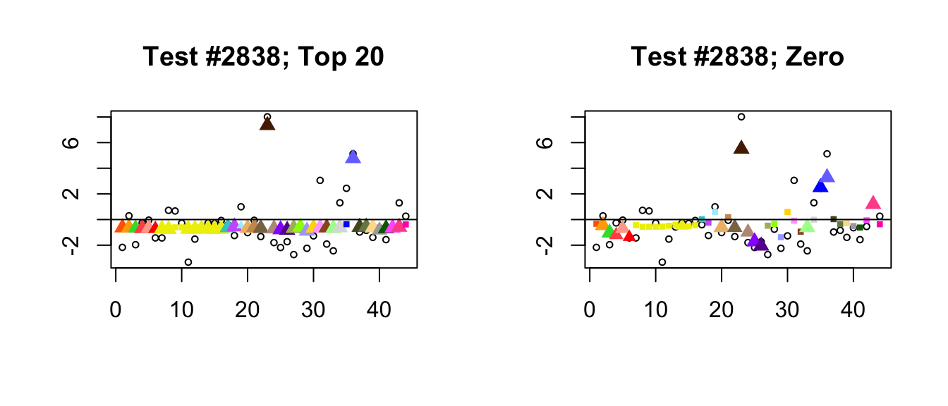
Expand here to see past versions of lg_uniq-1.png:
| Version | Author | Date |
|---|---|---|
| 1d57c08 | Jason Willwerscheid | 2018-08-04 |
Expand here to see past versions of lg_uniq-2.png:
| Version | Author | Date |
|---|---|---|
| 1d57c08 | Jason Willwerscheid | 2018-08-04 |
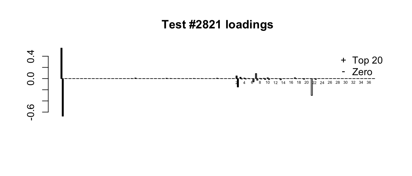
- In a second, infrequent class of cases, at least one of the additional 17 data-driven factors in the “Zero” fit turns out to be important. In the following example, the 21st loading, which quite plausibly introduces correlations among ovarian, uterine, and vaginal tissues (see here), has a moderate weight. This pushes the estimates for these tissues down just enough to make the effects more significant than effects in other non-brain tissues. As in the previous example, the “Top 20” fit has a much simpler interpretation: in this case, only the “equal effects” loading is important.
plot_it(2821)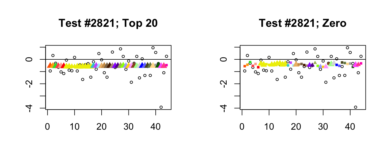
Expand here to see past versions of extra_dd-1.png:
| Version | Author | Date |
|---|---|---|
| 1d57c08 | Jason Willwerscheid | 2018-08-04 |
Expand here to see past versions of extra_dd-2.png:
| Version | Author | Date |
|---|---|---|
| 1d57c08 | Jason Willwerscheid | 2018-08-04 |
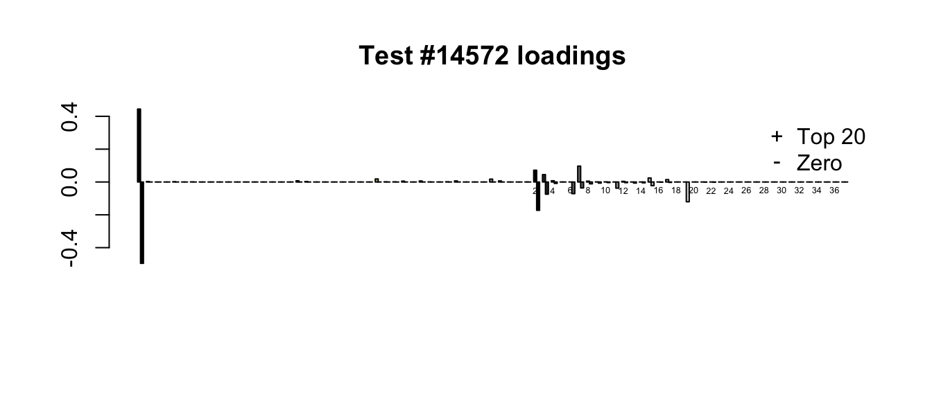
- Finally, there is a class of cases where posterior means are very similar but one method finds significance where the other does not. What’s happening, I think, is that because it does not include a canonical equal-effects loading, the “Zero” fit generally loads the second data-driven factor as well as the first. In other words, the “Zero” fit makes up for the absence of an equal-effects factor by combining the first two data-driven factors, which increases the degree of uncertainty in the point estimates.
plot_it(14572)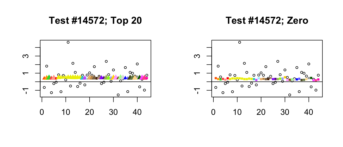
Expand here to see past versions of not_interpretable-1.png:
| Version | Author | Date |
|---|---|---|
| 1d57c08 | Jason Willwerscheid | 2018-08-04 |
Expand here to see past versions of not_interpretable-2.png:
| Version | Author | Date |
|---|---|---|
| 1d57c08 | Jason Willwerscheid | 2018-08-04 |
Significant for Zero, not Top 20
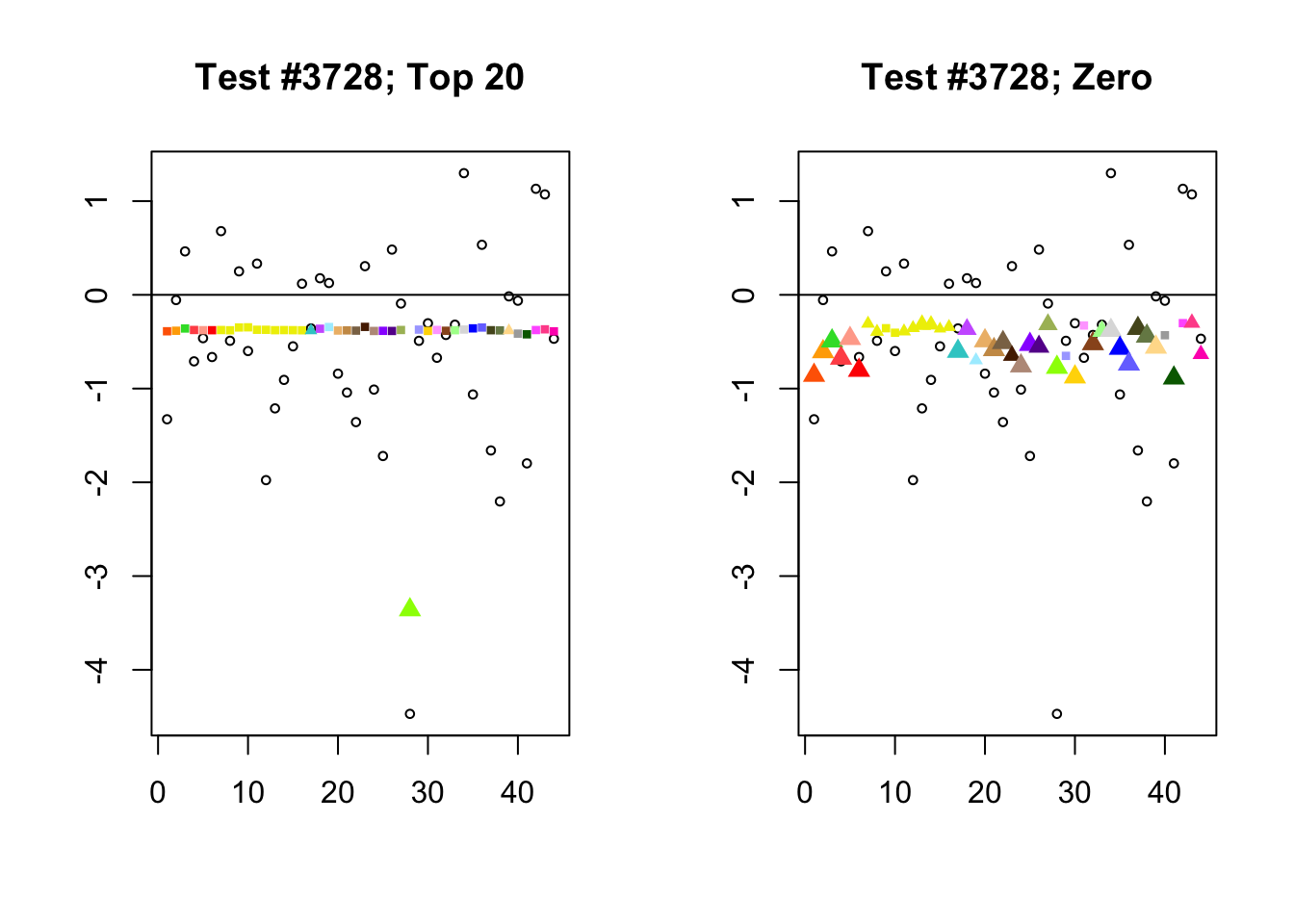
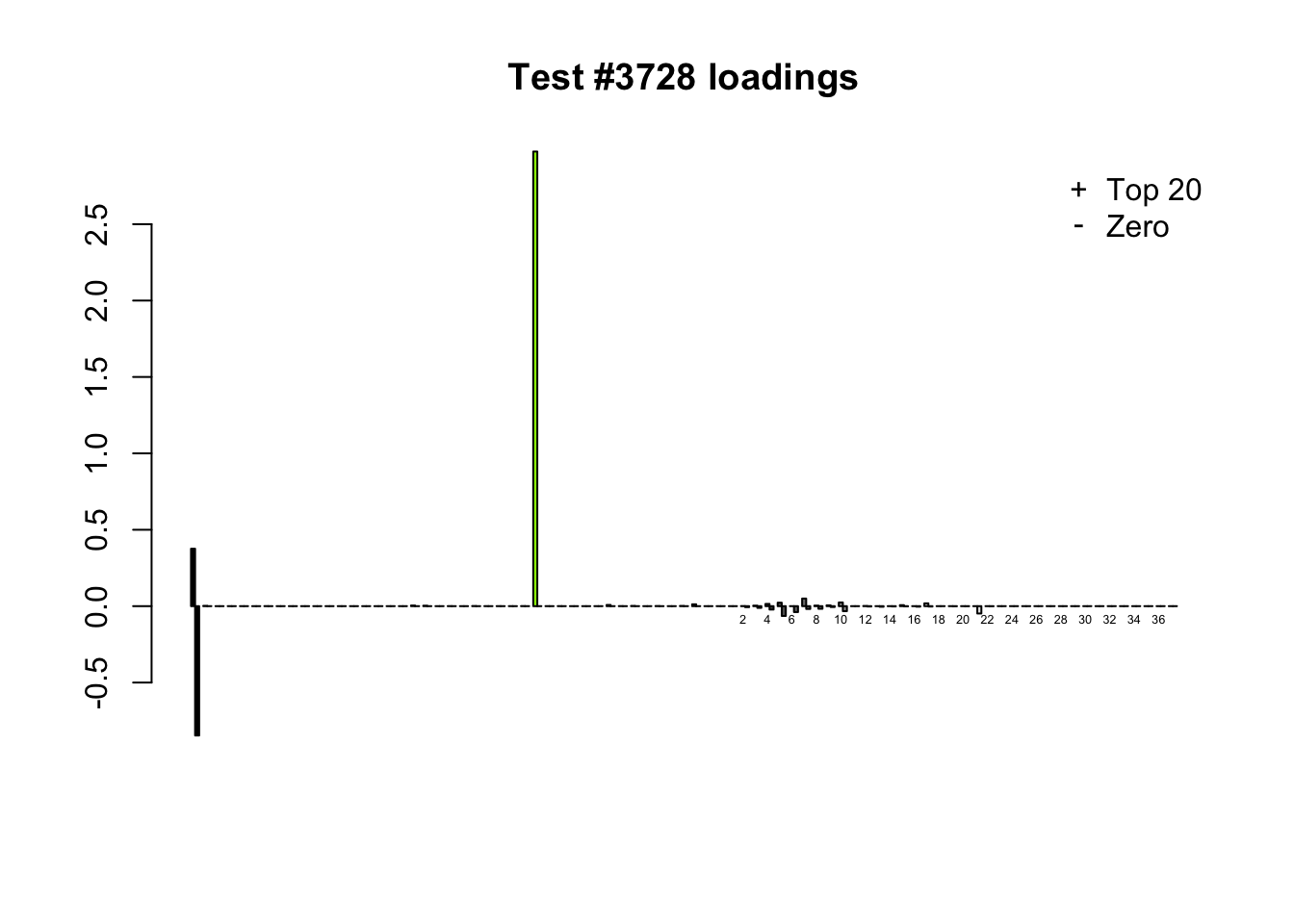
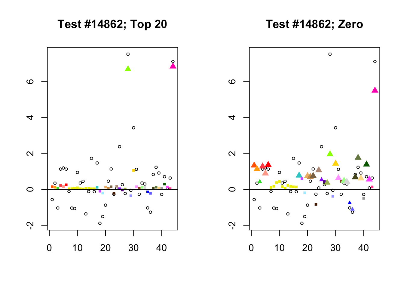
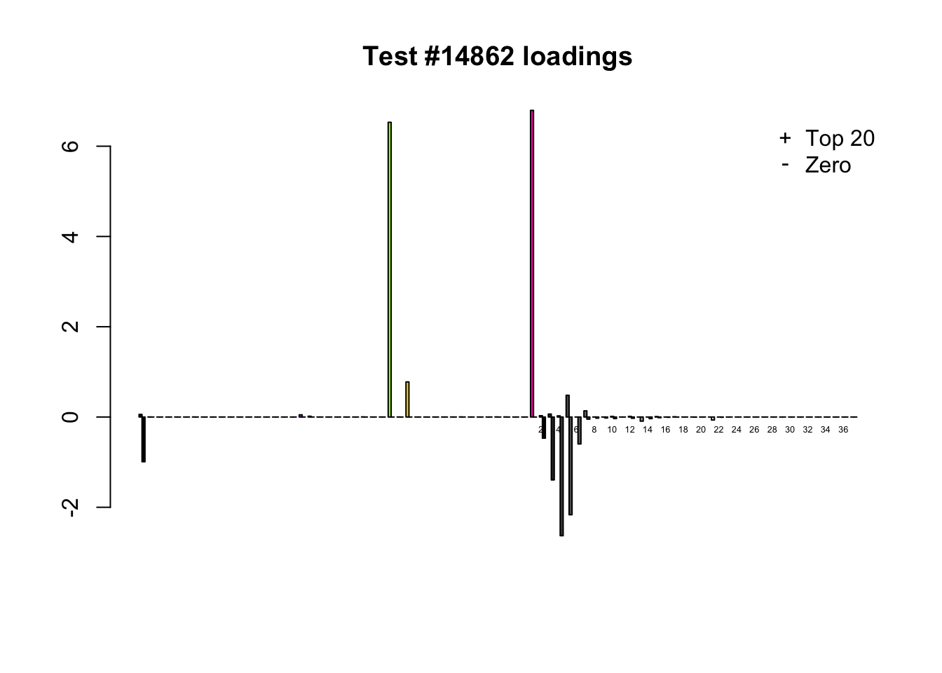
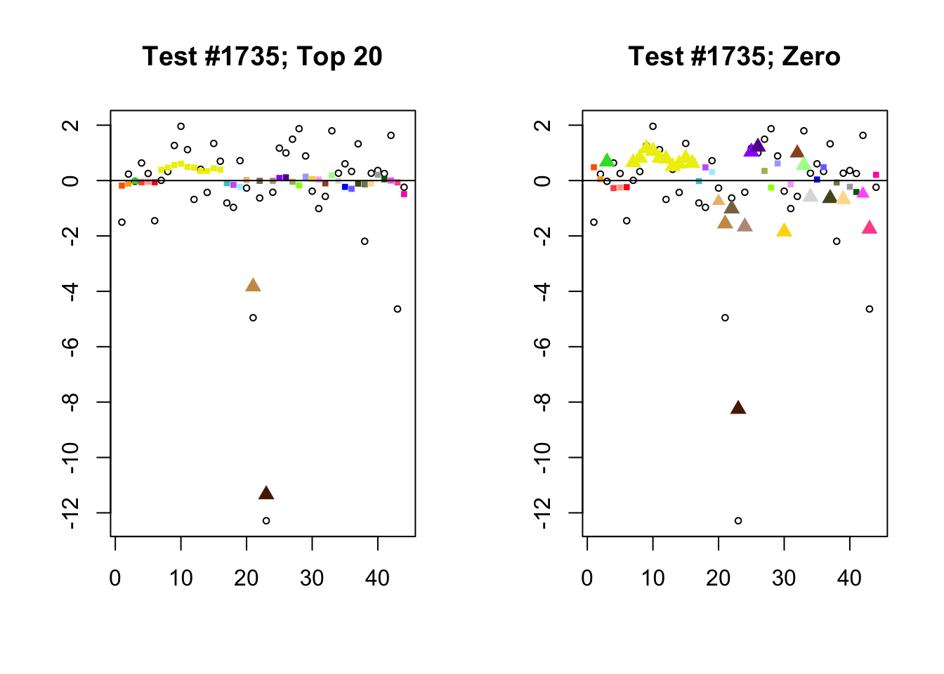
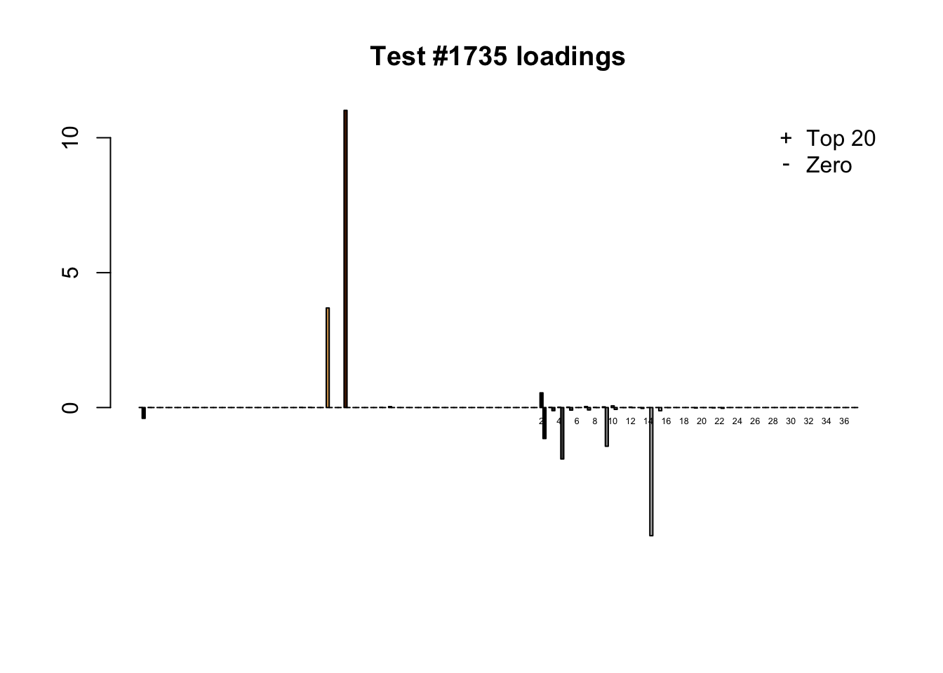
When the “Zero” method picks out significant effects but the “Top 20” method does not, the culprit is most often one or two outlying effects, as in the first class of cases discussed above. Three typical examples follow.
lg.uniq <- c(3728, 14862, 1735)
for (n in lg.uniq) {
  plot_it(n)
}
Expand here to see past versions of zero_not_top20-1.png:
| Version | Author | Date |
|---|---|---|
| 1d57c08 | Jason Willwerscheid | 2018-08-04 |
Expand here to see past versions of zero_not_top20-2.png:
| Version | Author | Date |
|---|---|---|
| 1d57c08 | Jason Willwerscheid | 2018-08-04 |
Expand here to see past versions of zero_not_top20-3.png:
| Version | Author | Date |
|---|---|---|
| 1d57c08 | Jason Willwerscheid | 2018-08-04 |
Expand here to see past versions of zero_not_top20-4.png:
| Version | Author | Date |
|---|---|---|
| 1d57c08 | Jason Willwerscheid | 2018-08-04 |
Expand here to see past versions of zero_not_top20-5.png:
| Version | Author | Date |
|---|---|---|
| 1d57c08 | Jason Willwerscheid | 2018-08-04 |
Expand here to see past versions of zero_not_top20-6.png:
| Version | Author | Date |
|---|---|---|
| 1d57c08 | Jason Willwerscheid | 2018-08-04 |
Different posterior means
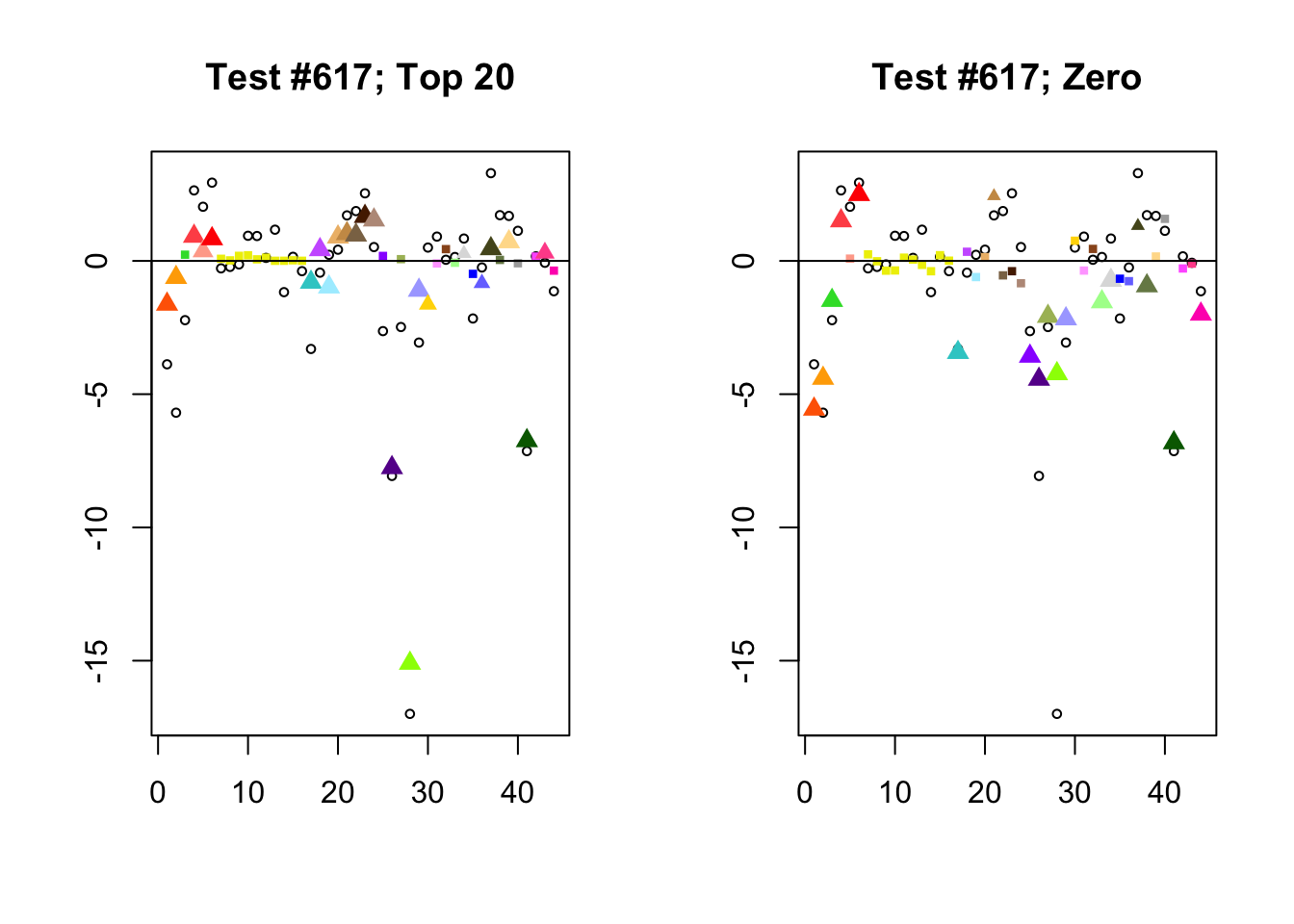
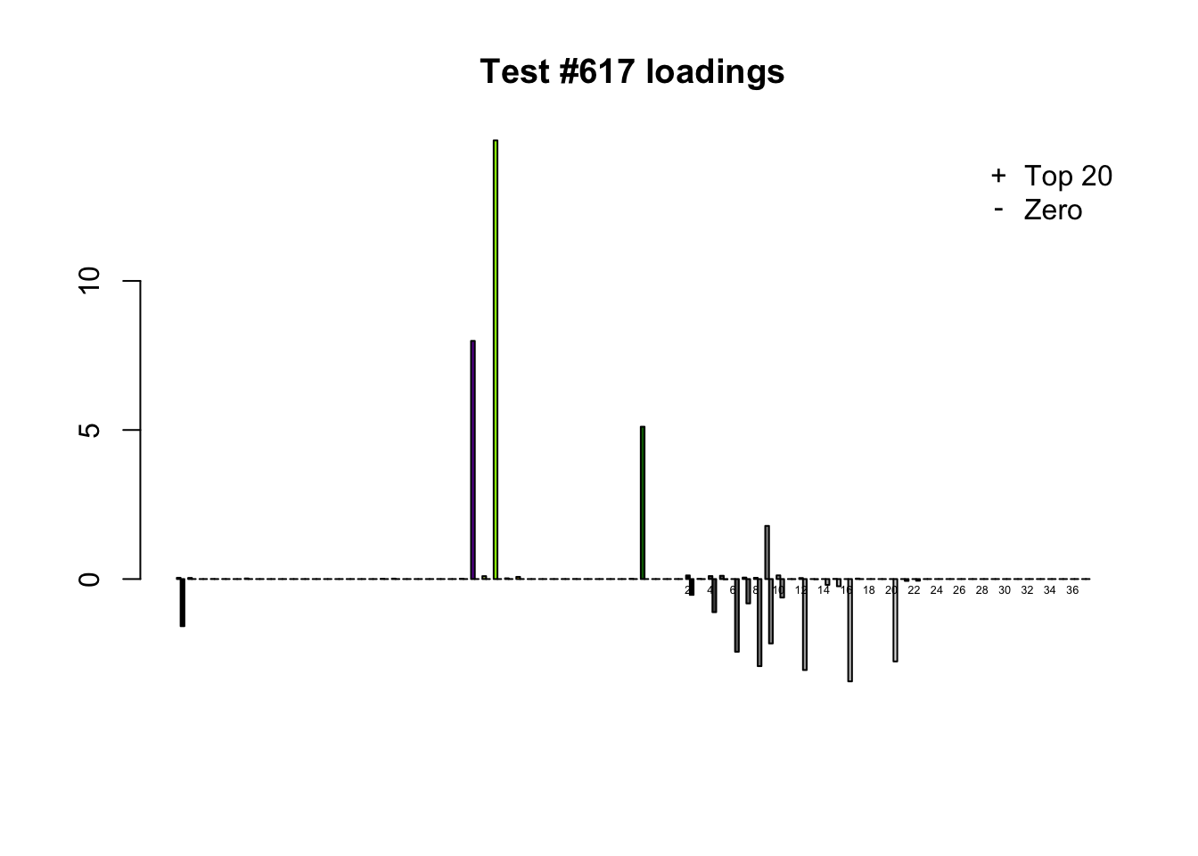
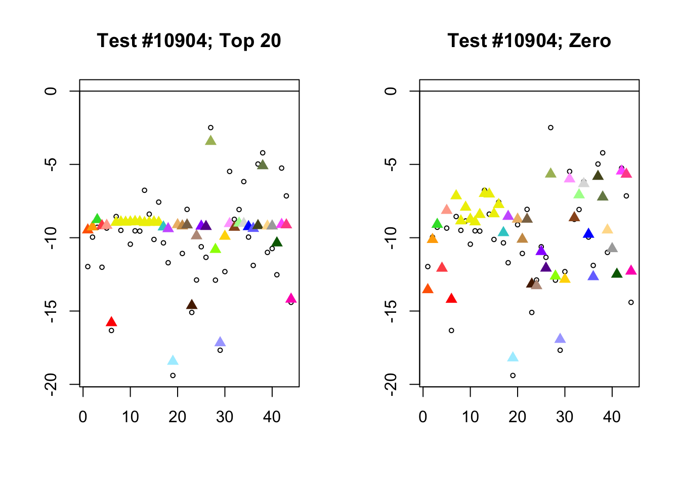
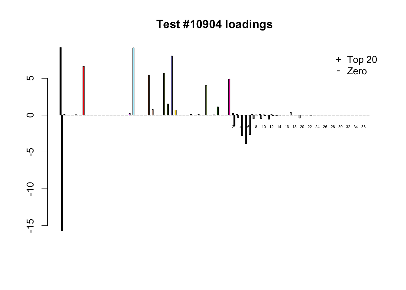
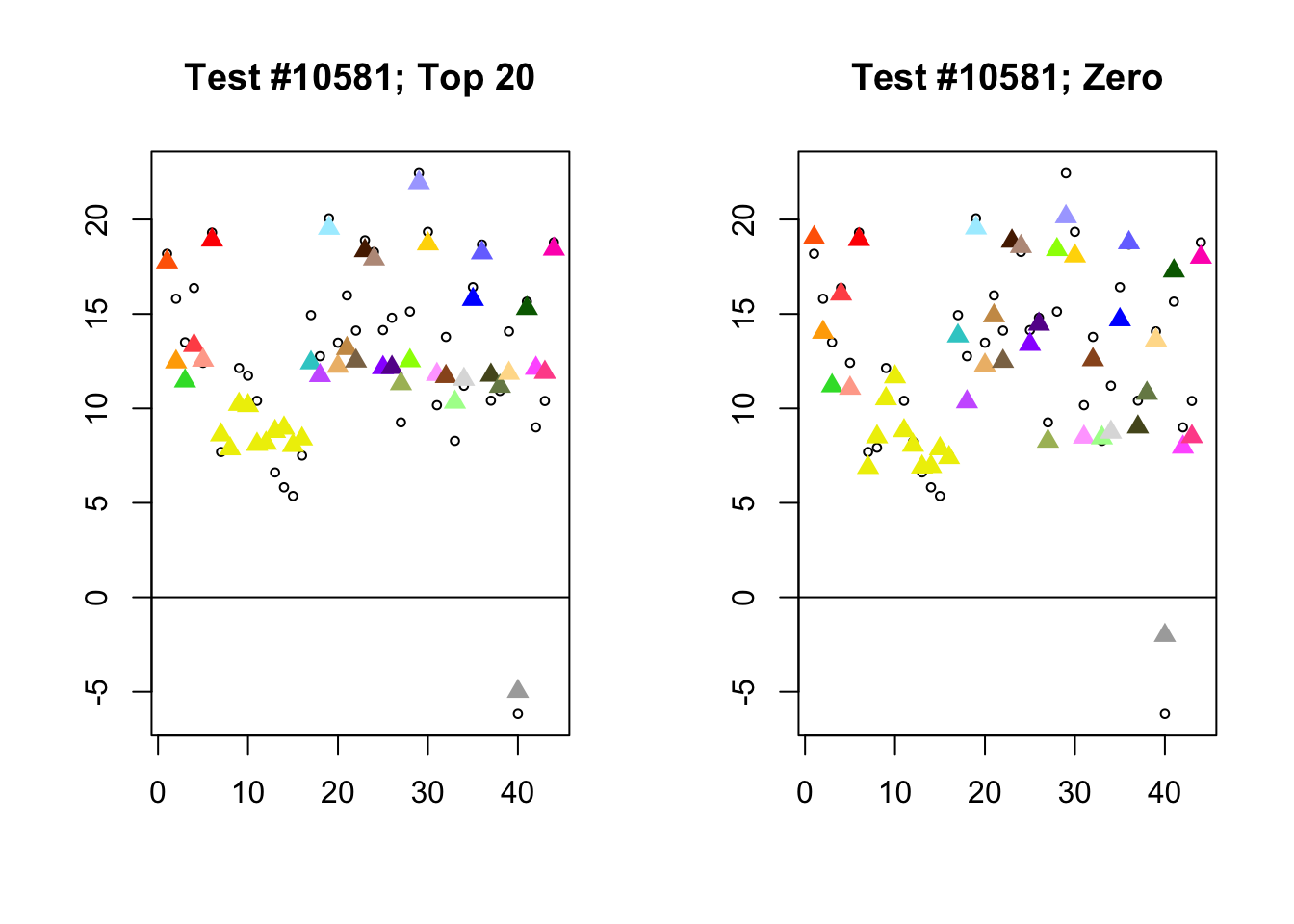
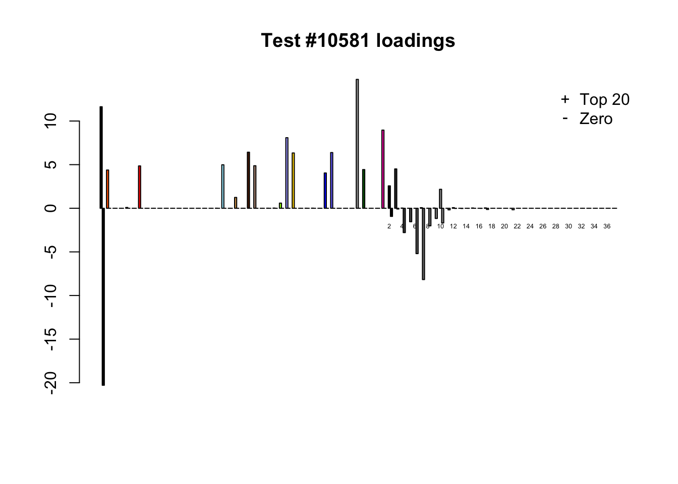
Each of the following examples illustrates how the additional canonical loadings can create large differences in posterior means (the extra data-driven loadings are unimportant in each case). It is difficult to generalize any further: sometimes the result is a small equal-effects loading (#617); sometimes, the data-driven loadings become unimportant, so that the comparatively smaller effects are aggressively shrunken towards their mean (#10904, #10581). I think that these examples point up one of the principal weaknesses of the “Zero” fit, which is that without the canonical loadings, many of the results become difficult to interpret (and therefore less plausible).
diff.pms <- c(617, 10904, 10581)
for (n in diff.pms) {
  plot_it(n)
}
Expand here to see past versions of diff_pms-1.png:
| Version | Author | Date |
|---|---|---|
| 1d57c08 | Jason Willwerscheid | 2018-08-04 |
Expand here to see past versions of diff_pms-2.png:
| Version | Author | Date |
|---|---|---|
| 1d57c08 | Jason Willwerscheid | 2018-08-04 |
Expand here to see past versions of diff_pms-3.png:
| Version | Author | Date |
|---|---|---|
| 1d57c08 | Jason Willwerscheid | 2018-08-04 |
Expand here to see past versions of diff_pms-4.png:
| Version | Author | Date |
|---|---|---|
| 1d57c08 | Jason Willwerscheid | 2018-08-04 |
Expand here to see past versions of diff_pms-5.png:
| Version | Author | Date |
|---|---|---|
| 1d57c08 | Jason Willwerscheid | 2018-08-04 |
Expand here to see past versions of diff_pms-6.png:
| Version | Author | Date |
|---|---|---|
| 1d57c08 | Jason Willwerscheid | 2018-08-04 |
Session information
sessionInfo()R version 3.4.3 (2017-11-30)
Platform: x86_64-apple-darwin15.6.0 (64-bit)
Running under: macOS High Sierra 10.13.6
Matrix products: default
BLAS: /Library/Frameworks/R.framework/Versions/3.4/Resources/lib/libRblas.0.dylib
LAPACK: /Library/Frameworks/R.framework/Versions/3.4/Resources/lib/libRlapack.dylib
locale:
[1] en_US.UTF-8/en_US.UTF-8/en_US.UTF-8/C/en_US.UTF-8/en_US.UTF-8
attached base packages:
[1] stats graphics grDevices utils datasets methods base
other attached packages:
[1] flashr_0.5-13 mashr_0.2-7 ashr_2.2-10
loaded via a namespace (and not attached):
[1] Rcpp_0.12.17 pillar_1.2.1 compiler_3.4.3
[4] git2r_0.21.0 plyr_1.8.4 workflowr_1.0.1
[7] R.methodsS3_1.7.1 R.utils_2.6.0 iterators_1.0.9
[10] tools_3.4.3 testthat_2.0.0 digest_0.6.15
[13] tibble_1.4.2 gtable_0.2.0 evaluate_0.10.1
[16] memoise_1.1.0 lattice_0.20-35 rlang_0.2.0
[19] Matrix_1.2-12 foreach_1.4.4 commonmark_1.4
[22] yaml_2.1.17 parallel_3.4.3 ebnm_0.1-12
[25] mvtnorm_1.0-7 xml2_1.2.0 withr_2.1.1.9000
[28] stringr_1.3.0 knitr_1.20 roxygen2_6.0.1.9000
[31] devtools_1.13.4 rprojroot_1.3-2 grid_3.4.3
[34] R6_2.2.2 rmarkdown_1.8 rmeta_3.0
[37] ggplot2_2.2.1 magrittr_1.5 whisker_0.3-2
[40] scales_0.5.0 backports_1.1.2 codetools_0.2-15
[43] htmltools_0.3.6 MASS_7.3-48 assertthat_0.2.0
[46] softImpute_1.4 colorspace_1.3-2 stringi_1.1.6
[49] lazyeval_0.2.1 munsell_0.4.3 doParallel_1.0.11
[52] pscl_1.5.2 truncnorm_1.0-8 SQUAREM_2017.10-1
[55] R.oo_1.21.0 This reproducible R Markdown analysis was created with workflowr 1.0.1