MASH v FLASH GTEx analysis: OHF v “Top 20”
Last updated: 2018-08-04
workflowr checks: (Click a bullet for more information)-
✔ R Markdown file: up-to-date
Great! Since the R Markdown file has been committed to the Git repository, you know the exact version of the code that produced these results.
-
✔ Environment: empty
Great job! The global environment was empty. Objects defined in the global environment can affect the analysis in your R Markdown file in unknown ways. For reproduciblity it’s best to always run the code in an empty environment.
-
✔ Seed:
set.seed(20180609)The command
set.seed(20180609)was run prior to running the code in the R Markdown file. Setting a seed ensures that any results that rely on randomness, e.g. subsampling or permutations, are reproducible. -
✔ Session information: recorded
Great job! Recording the operating system, R version, and package versions is critical for reproducibility.
-
Great! You are using Git for version control. Tracking code development and connecting the code version to the results is critical for reproducibility. The version displayed above was the version of the Git repository at the time these results were generated.✔ Repository version: 85bdd0b
Note that you need to be careful to ensure that all relevant files for the analysis have been committed to Git prior to generating the results (you can usewflow_publishorwflow_git_commit). workflowr only checks the R Markdown file, but you know if there are other scripts or data files that it depends on. Below is the status of the Git repository when the results were generated:
Note that any generated files, e.g. HTML, png, CSS, etc., are not included in this status report because it is ok for generated content to have uncommitted changes.Ignored files: Ignored: .DS_Store Ignored: .Rhistory Ignored: .Rproj.user/ Ignored: data/ Ignored: docs/.DS_Store Ignored: docs/images/.DS_Store Ignored: docs/images/.Rapp.history Ignored: output/.DS_Store Ignored: output/.Rapp.history Ignored: output/MASHvFLASHgtex/.DS_Store Ignored: output/MASHvFLASHsims/.DS_Store Ignored: output/MASHvFLASHsims/backfit/.DS_Store Ignored: output/MASHvFLASHsims/backfit/.Rapp.history Unstaged changes: Modified: code/gtexanalysis.R
Expand here to see past versions:
| File | Version | Author | Date | Message |
|---|---|---|---|---|
| Rmd | 85bdd0b | Jason Willwerscheid | 2018-08-04 | wflow_publish(c(“analysis/OHFvTop20.Rmd”, “analysis/index.Rmd”)) |
| html | 7758c2f | Jason Willwerscheid | 2018-08-04 | Build site. |
| Rmd | 312476b | Jason Willwerscheid | 2018-08-04 | wflow_publish(c(“analysis/OHFvTop20.Rmd”, “analysis/MASHvOHF.Rmd”, |
Introduction
This analysis compares the “OHF” FLASH fit to the “Top 20” FLASH fit. See here for fitting details.
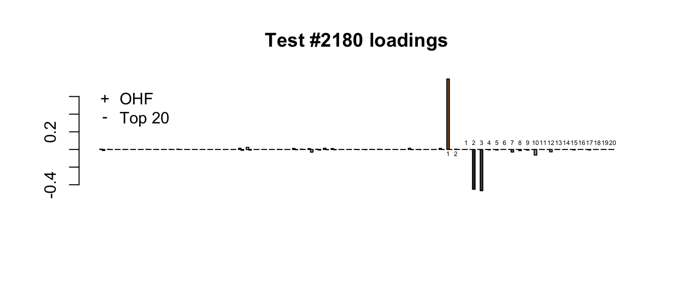
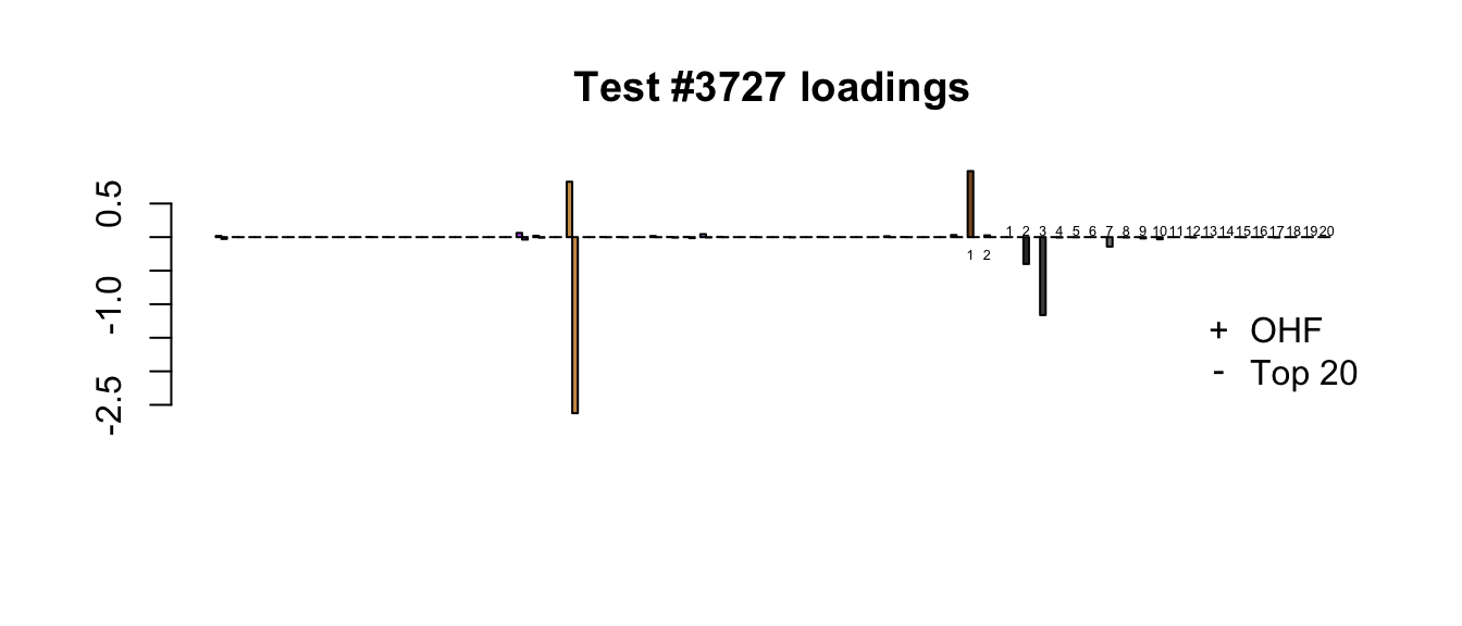
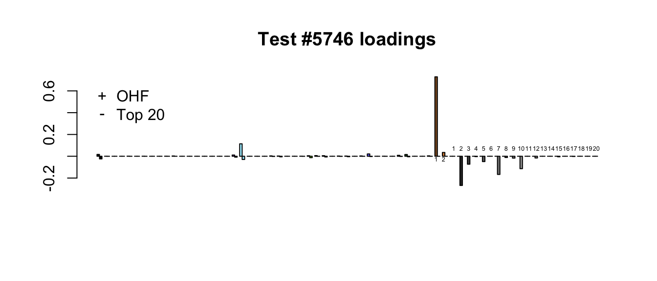
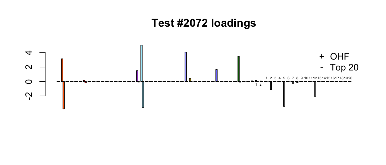
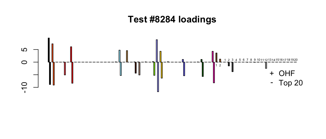
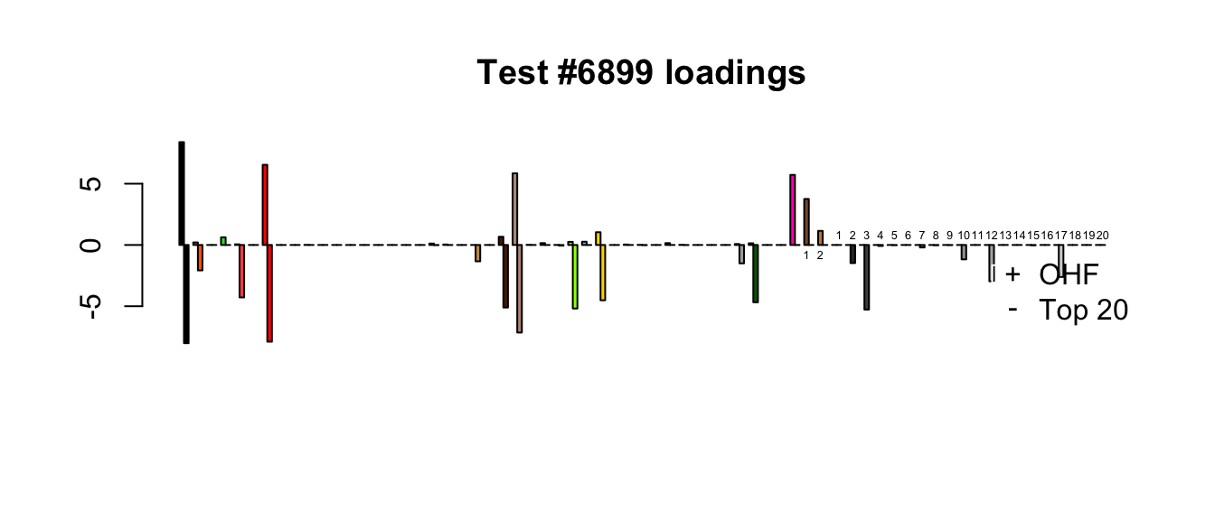
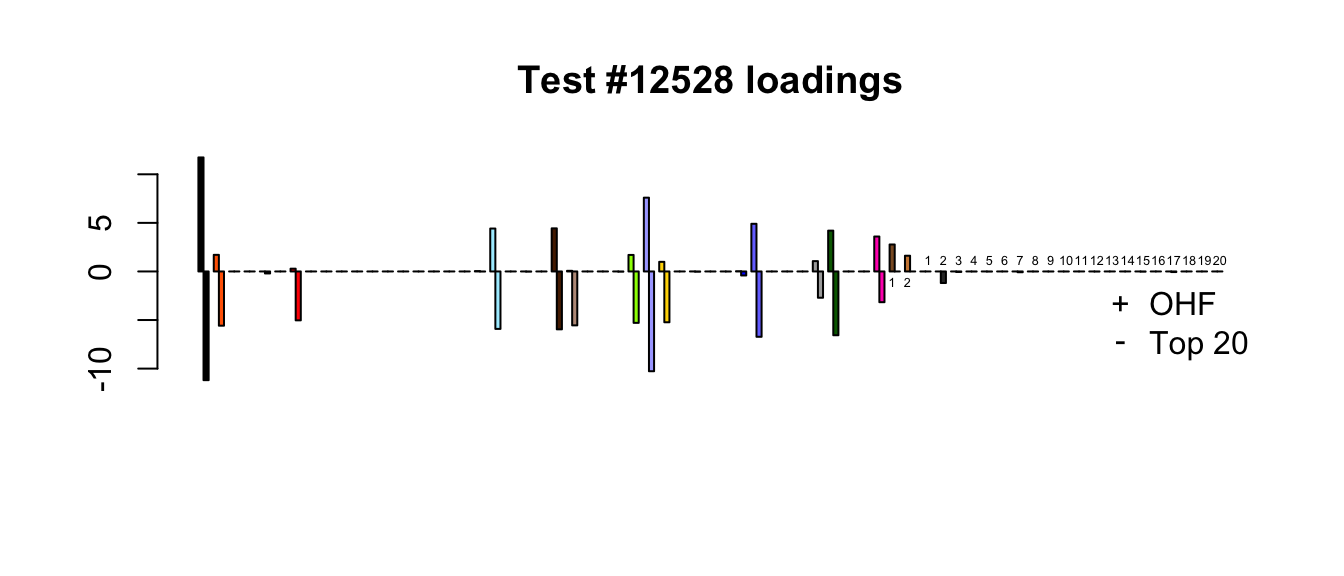
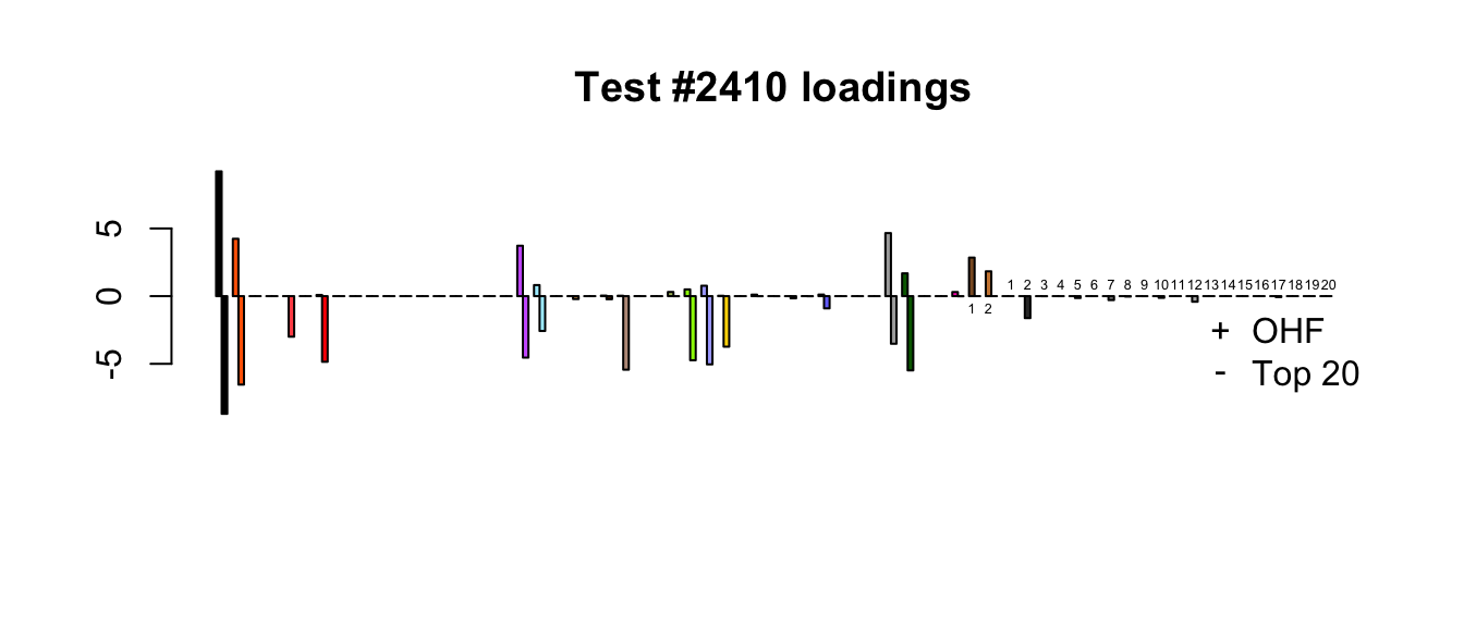
In general, differences among FLASH fits are much subtler than differences between the MASH fit and any given FLASH fit. To interpret the differences, I introduce a new plotting tool that compares loadings. Bar heights correspond to normalized absolute values of loadings, with loadings for the OHF method displayed above the x-axis and loadings for the “Top 20” method displayed below. The leftmost black bar corresponds to the “equal effects” loading; the colored bars correspond to unique effects; and the rightmost numbered bars correspond to data-driven loadings.
library(mashr)Loading required package: ashrdevtools::load_all("/Users/willwerscheid/GitHub/flashr/")Loading flashrgtex <- readRDS(gzcon(url("https://github.com/stephenslab/gtexresults/blob/master/data/MatrixEQTLSumStats.Portable.Z.rds?raw=TRUE")))
strong <- t(gtex$strong.z)
fpath <- "./output/MASHvFLASHgtex2/"
ohf_final <- readRDS(paste0(fpath, "ohf.rds"))
top20_final <- readRDS(paste0(fpath, "top20.rds"))
all_fl_lfsr <- readRDS(paste0(fpath, "fllfsr.rds"))
ohf_lfsr <- all_fl_lfsr[[1]]
top20_lfsr <- all_fl_lfsr[[4]]
ohf_pm <- flash_get_fitted_values(ohf_final)
top20_pm <- flash_get_fitted_values(top20_final)missing.tissues <- c(7, 8, 19, 20, 24, 25, 31, 34, 37)
gtex.colors <- read.table("https://github.com/stephenslab/gtexresults/blob/master/data/GTExColors.txt?raw=TRUE", sep = '\t', comment.char = '')[-missing.tissues, 2]
OHF.colors <- c("tan4", "tan3")
zero.colors <- c("black", gray.colors(19, 0.2, 0.9),
gray.colors(17, 0.95, 1))
plot_test <- function(n, lfsr, pm, method_name) {
plot(strong[, n], pch=1, col="black", xlab="", ylab="", cex=0.6,
ylim=c(min(c(strong[, n], 0)), max(c(strong[, n], 0))),
main=paste0("Test #", n, "; ", method_name))
size = rep(0.6, 44)
shape = rep(15, 44)
signif <- lfsr[, n] <= .05
shape[signif] <- 17
size[signif] <- 1.35 - 15 * lfsr[signif, n]
size <- pmin(size, 1.2)
points(pm[, n], pch=shape, col=as.character(gtex.colors), cex=size)
abline(0, 0)
}
plot_ohf_v_ohl_loadings <- function(n, ohf_fit, ohl_fit, ohl_name,
legend_pos = "bottomright") {
ohf <- abs(ohf_fit$EF[n, ] * apply(abs(ohf_fit$EL), 2, max))
ohl <- -abs(ohl_fit$EF[n, ] * apply(abs(ohl_fit$EL), 2, max))
data <- rbind(c(ohf, rep(0, length(ohl) - 45)),
c(ohl[1:45], rep(0, length(ohf) - 45),
ohl[46:length(ohl)]))
colors <- c("black",
as.character(gtex.colors),
OHF.colors,
zero.colors[1:(length(ohl) - 45)])
x <- barplot(data, beside=T, col=rep(colors, each=2),
main=paste0("Test #", n, " loadings"),
legend.text = c("OHF", ohl_name),
args.legend = list(x = legend_pos, bty = "n", pch="+-",
fill=NULL, border="white"))
text(x[2*(46:47) - 1], min(data) / 10,
labels=as.character(1:2), cex=0.4)
text(x[2*(48:ncol(data))], max(data) / 10,
labels=as.character(1:(length(ohl) - 45)), cex=0.4)
}
compare_methods <- function(lfsr1, lfsr2, pm1, pm2) {
res <- list()
res$first_not_second <- find_A_not_B(lfsr1, lfsr2)
res$lg_first_not_second <- find_large_A_not_B(lfsr1, lfsr2)
res$second_not_first <- find_A_not_B(lfsr2, lfsr1)
res$lg_second_not_first <- find_large_A_not_B(lfsr2, lfsr1)
res$diff_pms <- find_overall_pm_diff(pm1, pm2)
return(res)
}
# Find tests where many conditions are significant according to
# method A but not according to method B.
find_A_not_B <- function(lfsrA, lfsrB) {
select_tests(colSums(lfsrA <= 0.05 & lfsrB > 0.05))
}
# Find tests where many conditions are highly significant according to
# method A but are not significant according to method B.
find_large_A_not_B <- function(lfsrA, lfsrB) {
select_tests(colSums(lfsrA <= 0.01 & lfsrB > 0.05))
}
find_overall_pm_diff <- function(pmA, pmB, n = 4) {
pm_diff <- colSums((pmA - pmB)^2)
return(order(pm_diff, decreasing = TRUE)[1:4])
}
# Get at least four (or min_n) "top" tests.
select_tests <- function(colsums, min_n = 4) {
n <- 45
n_tests <- 0
while (n_tests < min_n && n > 0) {
n <- n - 1
n_tests <- sum(colsums >= n)
}
return(which(colsums >= n))
}plot_it <- function(n, legend.pos = "bottomright") {
par(mfrow=c(1, 2))
plot_test(n, ohf_lfsr, ohf_pm, "OHF")
plot_test(n, top20_lfsr, top20_pm, "Top 20")
par(mfrow=c(1, 1))
plot_ohf_v_ohl_loadings(n, ohf_final, top20_final, "Top 20",
legend.pos)
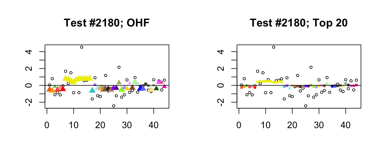
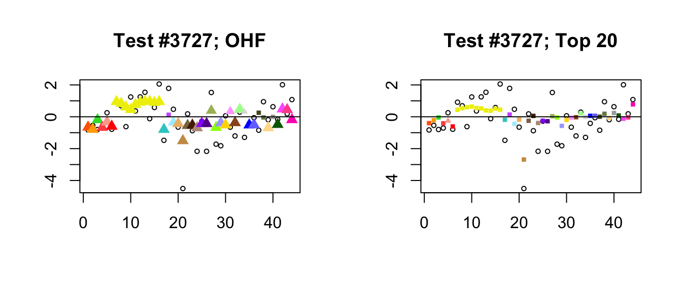
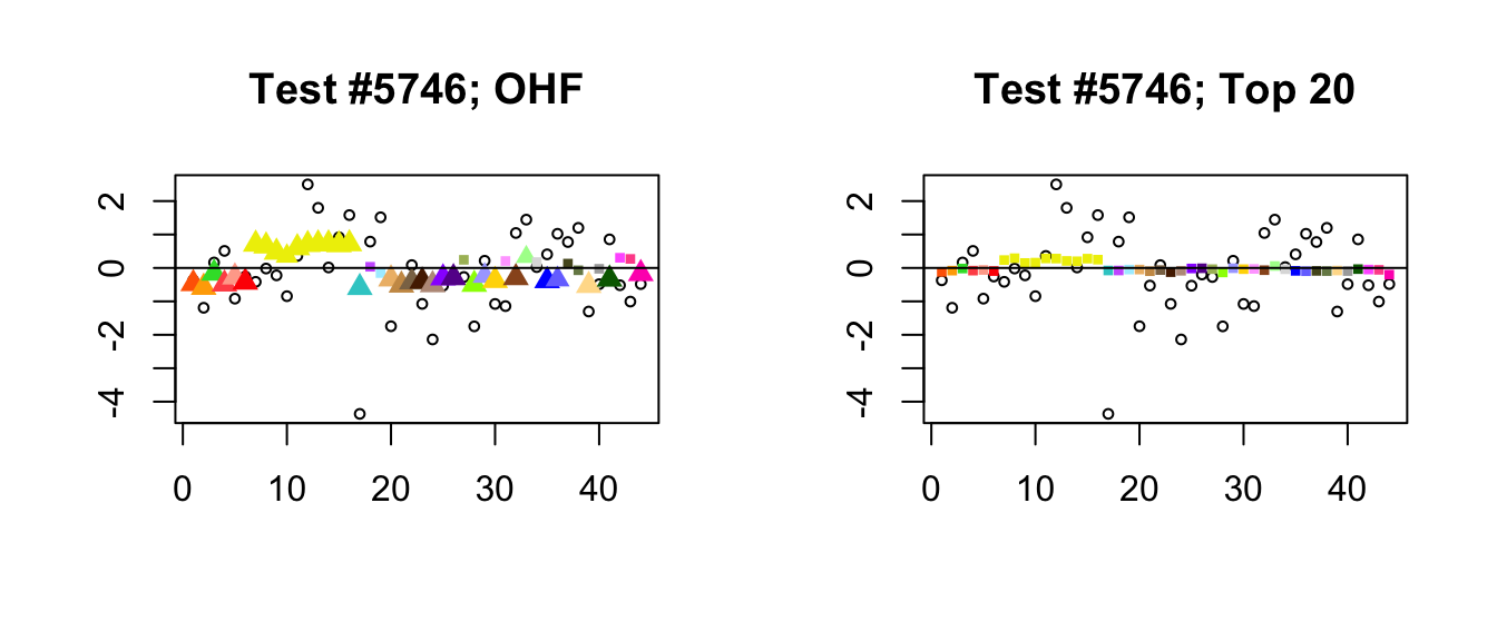
}Significant for OHF, not Top 20
The fact that the OHF fit only has two data-driven loadings can constrain its estimates to follow the patterns prescribed by those loadings (depicted here). Typically, when estimates are deemed significant by OHF but not by the “Top 20” method, OHF places a large weight on a single data-driven loading, whereas the “Top 20” method disperses weight across several data-driven loadings. The following examples are typical.
# ohf.v.top20 <- compare_methods(ohf_lfsr, top20_lfsr, ohf_pm, top20_pm)

ohl.first.loading <- c(2180, 3727, 5746)
legend.pos <- c("topleft", "bottomright", "topleft")
for (i in 1:length(ohl.first.loading)) {
  plot_it(ohl.first.loading[i], legend.pos[i])
}
Expand here to see past versions of ohf_not_mash-1.png:
| Version | Author | Date |
|---|---|---|
| 7758c2f | Jason Willwerscheid | 2018-08-04 |
Expand here to see past versions of ohf_not_mash-2.png:
| Version | Author | Date |
|---|---|---|
| 7758c2f | Jason Willwerscheid | 2018-08-04 |
Expand here to see past versions of ohf_not_mash-3.png:
| Version | Author | Date |
|---|---|---|
| 7758c2f | Jason Willwerscheid | 2018-08-04 |
Expand here to see past versions of ohf_not_mash-4.png:
| Version | Author | Date |
|---|---|---|
| 7758c2f | Jason Willwerscheid | 2018-08-04 |
Expand here to see past versions of ohf_not_mash-5.png:
| Version | Author | Date |
|---|---|---|
| 7758c2f | Jason Willwerscheid | 2018-08-04 |
Expand here to see past versions of ohf_not_mash-6.png:
| Version | Author | Date |
|---|---|---|
| 7758c2f | Jason Willwerscheid | 2018-08-04 |
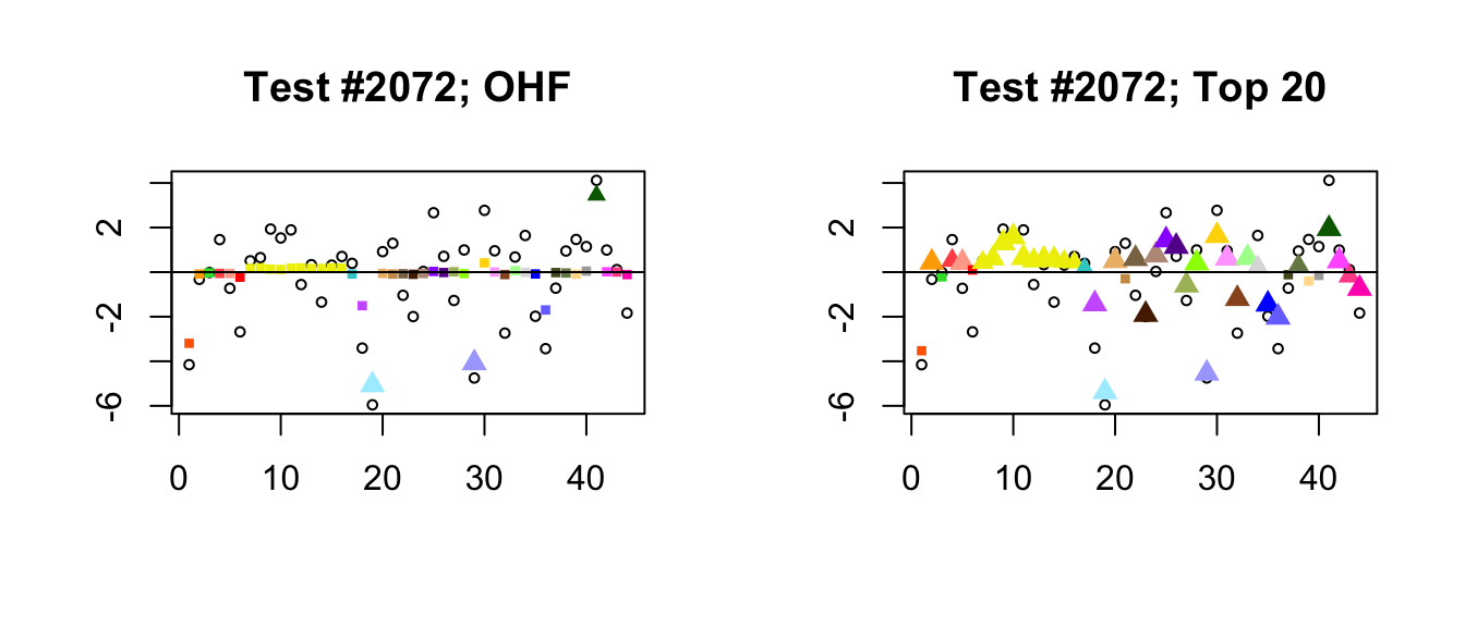
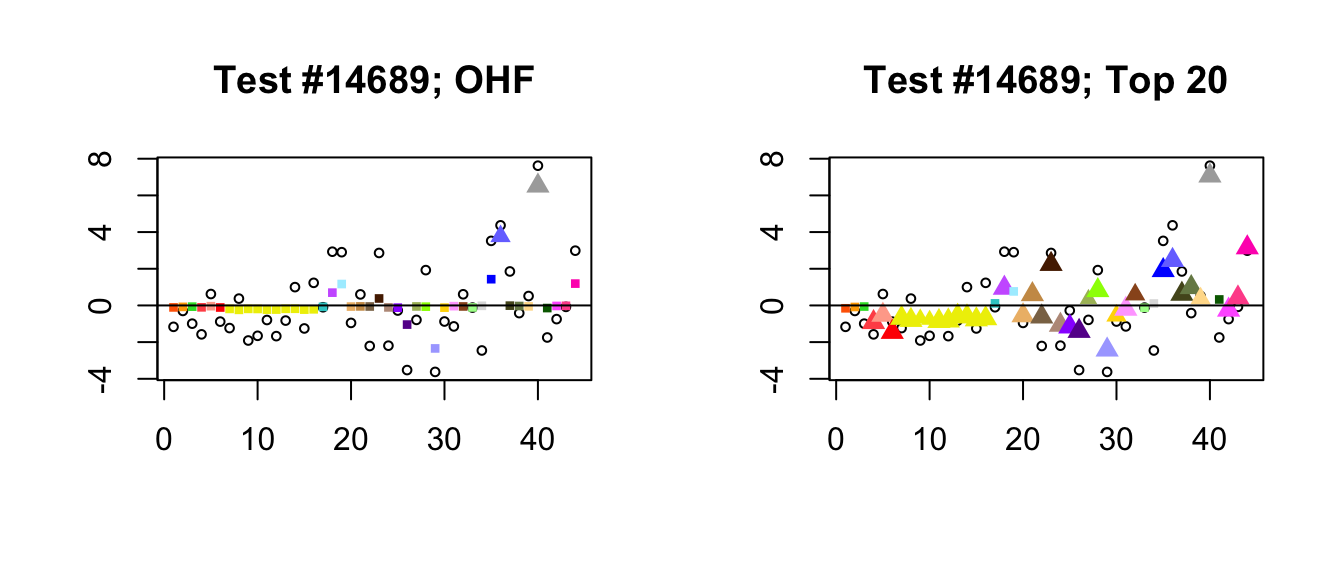
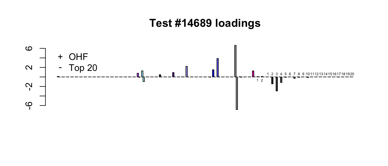
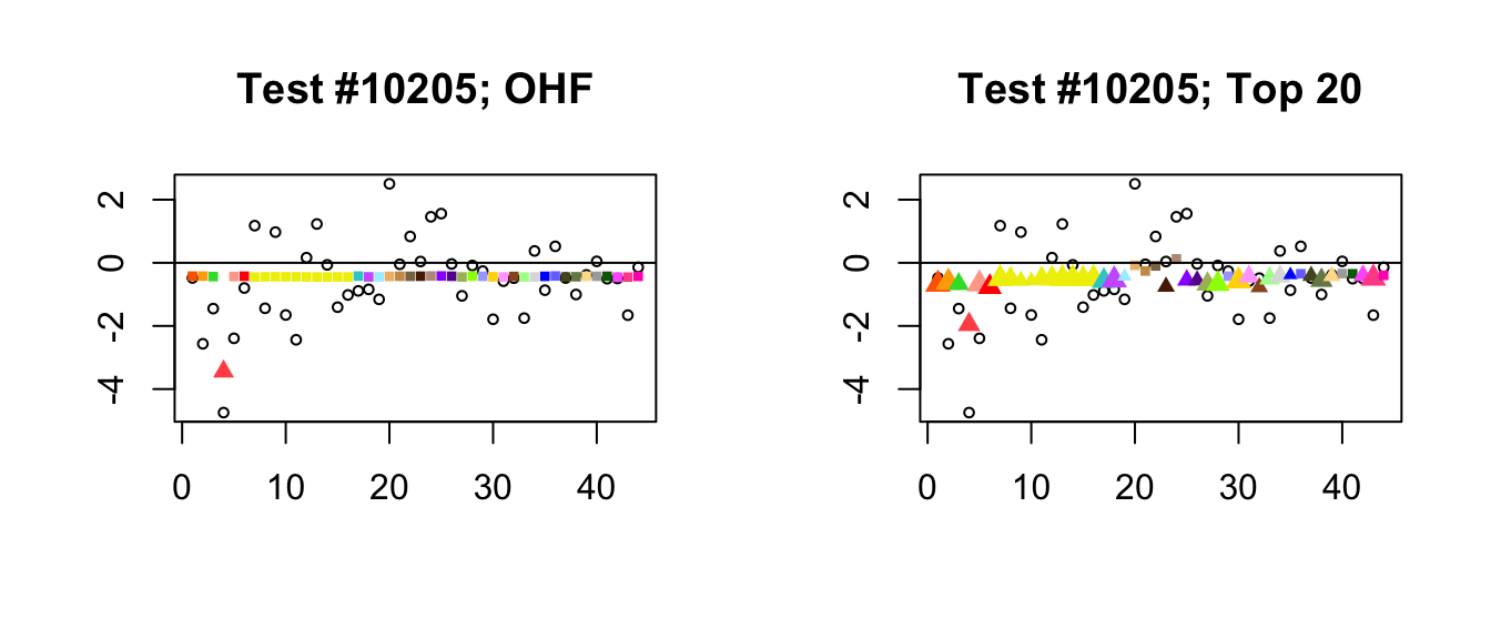
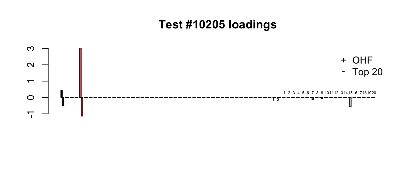
Significant for Top 20, not OHF
Another consequence of the fact that the OHF fit only has two data-driven loadings is that it will fail to find any patterns that are not prescribed by those loadings. In the following examples, OHF places virtually no weight on its data-driven loadings, whereas the “Top 20” method places moderate to large weights on at least a few data-driven loadings.
ohf.no.dd <- c(2072, 14689, 10205)
legend.pos <- c("topright", "topleft", "topright")
for (i in 1:length(ohf.no.dd)) {
  plot_it(ohf.no.dd[i], legend.pos[i])
}
Expand here to see past versions of mash_not_ohf-1.png:
| Version | Author | Date |
|---|---|---|
| 7758c2f | Jason Willwerscheid | 2018-08-04 |
Expand here to see past versions of mash_not_ohf-2.png:
| Version | Author | Date |
|---|---|---|
| 7758c2f | Jason Willwerscheid | 2018-08-04 |
Expand here to see past versions of mash_not_ohf-3.png:
| Version | Author | Date |
|---|---|---|
| 7758c2f | Jason Willwerscheid | 2018-08-04 |
Expand here to see past versions of mash_not_ohf-4.png:
| Version | Author | Date |
|---|---|---|
| 7758c2f | Jason Willwerscheid | 2018-08-04 |
Expand here to see past versions of mash_not_ohf-5.png:
| Version | Author | Date |
|---|---|---|
| 7758c2f | Jason Willwerscheid | 2018-08-04 |
Expand here to see past versions of mash_not_ohf-6.png:
| Version | Author | Date |
|---|---|---|
| 7758c2f | Jason Willwerscheid | 2018-08-04 |
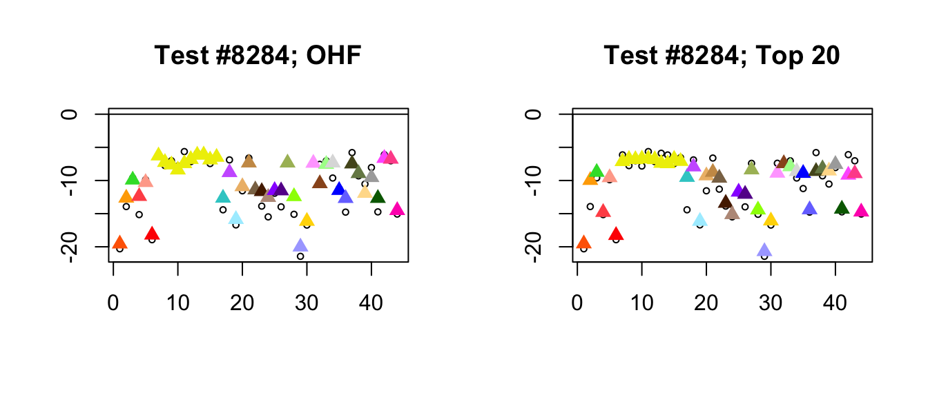
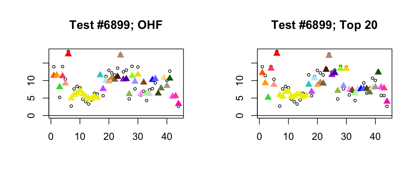
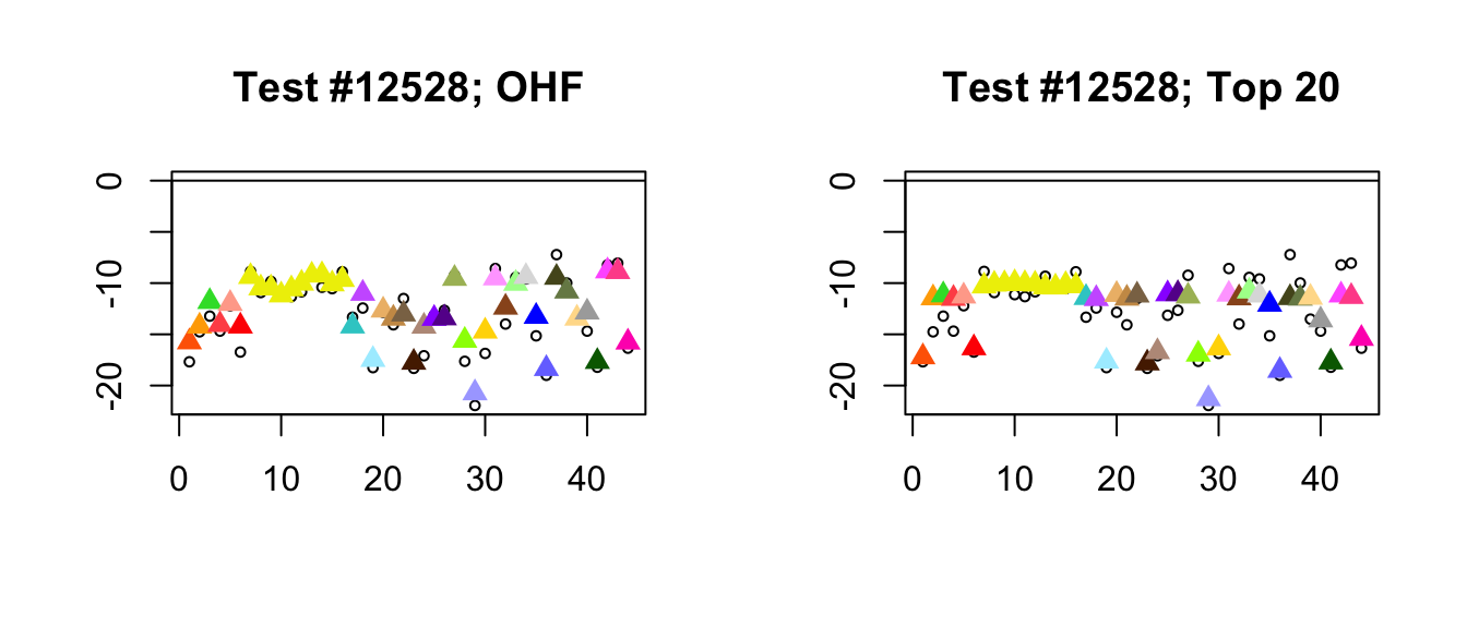
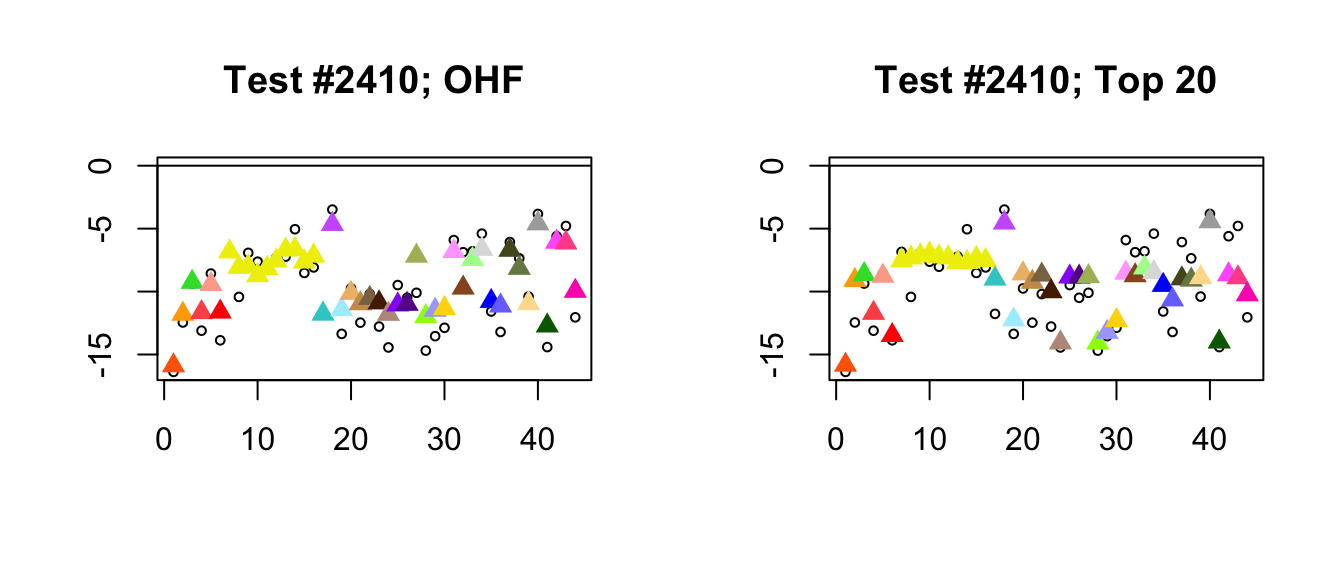
Different posterior means
This category of tests is perhaps the most intriguing of the three. In each of the following examples, the “Top 20” method assigns much larger weights to many unique effects, so that there is in general less shrinkage for the largest effects. As a result, it is also able to shrink the relatively smaller effects more aggressively.
diff.pms <- c(8284, 6899, 12528, 2410)
for (i in 1:length(diff.pms)) {
  plot_it(diff.pms[i])
}
Expand here to see past versions of diff_pms-1.png:
| Version | Author | Date |
|---|---|---|
| 7758c2f | Jason Willwerscheid | 2018-08-04 |
Expand here to see past versions of diff_pms-2.png:
| Version | Author | Date |
|---|---|---|
| 7758c2f | Jason Willwerscheid | 2018-08-04 |
Expand here to see past versions of diff_pms-3.png:
| Version | Author | Date |
|---|---|---|
| 7758c2f | Jason Willwerscheid | 2018-08-04 |
Expand here to see past versions of diff_pms-4.png:
| Version | Author | Date |
|---|---|---|
| 7758c2f | Jason Willwerscheid | 2018-08-04 |
Expand here to see past versions of diff_pms-5.png:
| Version | Author | Date |
|---|---|---|
| 7758c2f | Jason Willwerscheid | 2018-08-04 |
Expand here to see past versions of diff_pms-6.png:
| Version | Author | Date |
|---|---|---|
| 7758c2f | Jason Willwerscheid | 2018-08-04 |
Expand here to see past versions of diff_pms-7.png:
| Version | Author | Date |
|---|---|---|
| 7758c2f | Jason Willwerscheid | 2018-08-04 |
Expand here to see past versions of diff_pms-8.png:
| Version | Author | Date |
|---|---|---|
| 7758c2f | Jason Willwerscheid | 2018-08-04 |
Session information
sessionInfo()R version 3.4.3 (2017-11-30)
Platform: x86_64-apple-darwin15.6.0 (64-bit)
Running under: macOS High Sierra 10.13.6
Matrix products: default
BLAS: /Library/Frameworks/R.framework/Versions/3.4/Resources/lib/libRblas.0.dylib
LAPACK: /Library/Frameworks/R.framework/Versions/3.4/Resources/lib/libRlapack.dylib
locale:
[1] en_US.UTF-8/en_US.UTF-8/en_US.UTF-8/C/en_US.UTF-8/en_US.UTF-8
attached base packages:
[1] stats graphics grDevices utils datasets methods base
other attached packages:
[1] flashr_0.5-12 mashr_0.2-7 ashr_2.2-10
loaded via a namespace (and not attached):
[1] Rcpp_0.12.17 pillar_1.2.1 compiler_3.4.3
[4] git2r_0.21.0 plyr_1.8.4 workflowr_1.0.1
[7] R.methodsS3_1.7.1 R.utils_2.6.0 iterators_1.0.9
[10] tools_3.4.3 testthat_2.0.0 digest_0.6.15
[13] tibble_1.4.2 gtable_0.2.0 evaluate_0.10.1
[16] memoise_1.1.0 lattice_0.20-35 rlang_0.2.0
[19] Matrix_1.2-12 foreach_1.4.4 commonmark_1.4
[22] yaml_2.1.17 parallel_3.4.3 ebnm_0.1-12
[25] mvtnorm_1.0-7 xml2_1.2.0 withr_2.1.1.9000
[28] stringr_1.3.0 knitr_1.20 roxygen2_6.0.1.9000
[31] devtools_1.13.4 rprojroot_1.3-2 grid_3.4.3
[34] R6_2.2.2 rmarkdown_1.8 rmeta_3.0
[37] ggplot2_2.2.1 magrittr_1.5 whisker_0.3-2
[40] scales_0.5.0 backports_1.1.2 codetools_0.2-15
[43] htmltools_0.3.6 MASS_7.3-48 assertthat_0.2.0
[46] softImpute_1.4 colorspace_1.3-2 stringi_1.1.6
[49] lazyeval_0.2.1 munsell_0.4.3 doParallel_1.0.11
[52] pscl_1.5.2 truncnorm_1.0-8 SQUAREM_2017.10-1
[55] R.oo_1.21.0 This reproducible R Markdown analysis was created with workflowr 1.0.1