MASH v FLASH GTEx analysis: MASH v OHF
Last updated: 2018-08-04
workflowr checks: (Click a bullet for more information)-
✔ R Markdown file: up-to-date
Great! Since the R Markdown file has been committed to the Git repository, you know the exact version of the code that produced these results.
-
✔ Environment: empty
Great job! The global environment was empty. Objects defined in the global environment can affect the analysis in your R Markdown file in unknown ways. For reproduciblity it’s best to always run the code in an empty environment.
-
✔ Seed:
set.seed(20180609)The command
set.seed(20180609)was run prior to running the code in the R Markdown file. Setting a seed ensures that any results that rely on randomness, e.g. subsampling or permutations, are reproducible. -
✔ Session information: recorded
Great job! Recording the operating system, R version, and package versions is critical for reproducibility.
-
Great! You are using Git for version control. Tracking code development and connecting the code version to the results is critical for reproducibility. The version displayed above was the version of the Git repository at the time these results were generated.✔ Repository version: 312476b
Note that you need to be careful to ensure that all relevant files for the analysis have been committed to Git prior to generating the results (you can usewflow_publishorwflow_git_commit). workflowr only checks the R Markdown file, but you know if there are other scripts or data files that it depends on. Below is the status of the Git repository when the results were generated:
Note that any generated files, e.g. HTML, png, CSS, etc., are not included in this status report because it is ok for generated content to have uncommitted changes.Ignored files: Ignored: .DS_Store Ignored: .Rhistory Ignored: .Rproj.user/ Ignored: data/ Ignored: docs/.DS_Store Ignored: docs/images/.DS_Store Ignored: docs/images/.Rapp.history Ignored: output/.DS_Store Ignored: output/.Rapp.history Ignored: output/MASHvFLASHgtex/.DS_Store Ignored: output/MASHvFLASHsims/.DS_Store Ignored: output/MASHvFLASHsims/backfit/.DS_Store Ignored: output/MASHvFLASHsims/backfit/.Rapp.history Untracked files: Untracked: docs/figure/OHFvTop20.Rmd/ Unstaged changes: Modified: code/gtexanalysis.R
Expand here to see past versions:
| File | Version | Author | Date | Message |
|---|---|---|---|---|
| html | 5401954 | Jason Willwerscheid | 2018-08-04 | Build site. |
| Rmd | b2aa853 | Jason Willwerscheid | 2018-08-04 | wflow_publish(c(“analysis/MASHvTop20.Rmd”, |
| html | ea857fe | Jason Willwerscheid | 2018-08-03 | Build site. |
| Rmd | c5d0c86 | Jason Willwerscheid | 2018-08-03 | wflow_publish(“analysis/MASHvOHF.Rmd”) |
| html | e78875c | Jason Willwerscheid | 2018-08-02 | Build site. |
| Rmd | 0e165ca | Jason Willwerscheid | 2018-08-02 | wflow_publish(c(“analysis/MASHvOHF.Rmd”, “analysis/index.Rmd”)) |
| html | a91ab89 | Jason Willwerscheid | 2018-08-02 | Build site. |
| Rmd | cebcb57 | Jason Willwerscheid | 2018-08-02 | wflow_publish(“analysis/MASHvOHF.Rmd”) |
Introduction
In the previous analysis, I proposed several workflows for fitting MASH and FLASH objects to GTEx data. Here and in the next few analyses I examine differences among fits. I begin by comparing the MASH fit to the OHF fit.
For the code used to obtain the fits, see the previous analysis.
library(mashr)Loading required package: ashrdevtools::load_all("/Users/willwerscheid/GitHub/flashr/")Loading flashrgtex <- readRDS(gzcon(url("https://github.com/stephenslab/gtexresults/blob/master/data/MatrixEQTLSumStats.Portable.Z.rds?raw=TRUE")))
strong <- t(gtex$strong.z)
fpath <- "./output/MASHvFLASHgtex2/"
m_final <- readRDS(paste0(fpath, "m.rds"))
fl_final <- readRDS(paste0(fpath, "OHF.rds"))
m_lfsr <- t(get_lfsr(m_final))
m_pm <- t(get_pm(m_final))
fl_lfsr <- readRDS(paste0(fpath, "fllfsr.rds"))
fl_lfsr <- fl_lfsr[[1]]
fl_pm <- flash_get_fitted_values(fl_final)Introduction to plots
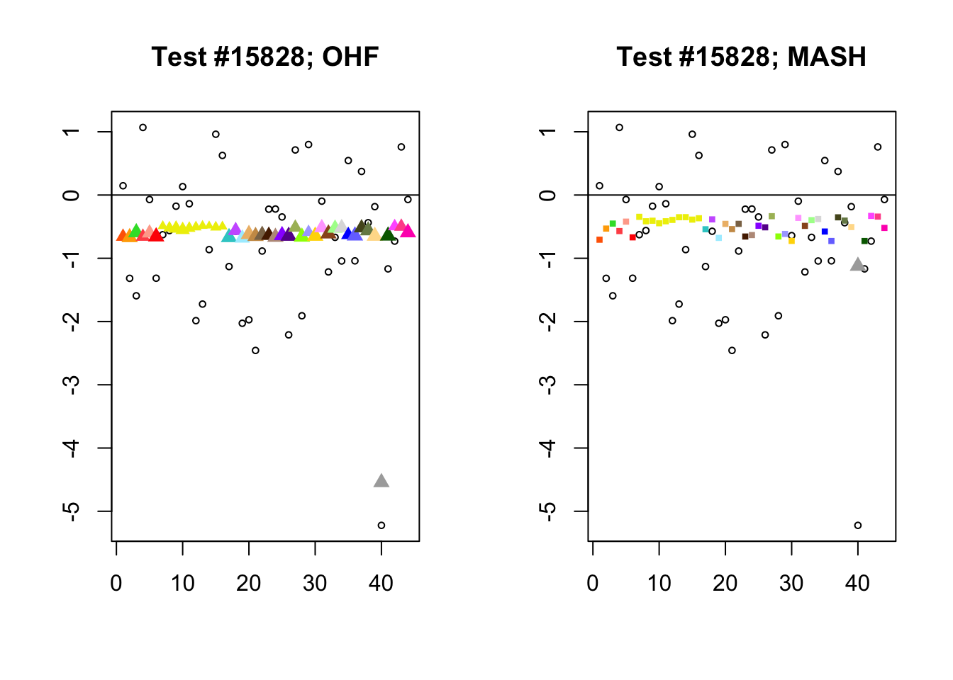
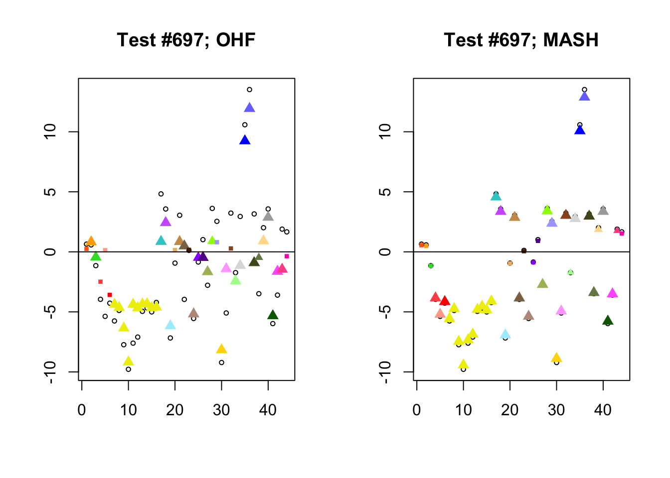
The main tool I will use in these analyses is a function that plots observed values vs. MASH or FLASH posterior means for a single test (over all 44 conditions).
The observed \(z\)-scores are plotted as hollow circles. Posterior means are plotted as triangles if the effect is judged to be significant (LFSR \(\le .05\)) and as squares otherwise. Larger triangles indicate lower LFSRs, with the largest triangles corresponding to “highly significant” effects (LFSR \(\le .01\)). The posterior means are colored using the GTEx colors used in previous analyses.
missing.tissues <- c(7, 8, 19, 20, 24, 25, 31, 34, 37)
gtex.colors <- read.table("https://github.com/stephenslab/gtexresults/blob/master/data/GTExColors.txt?raw=TRUE", sep = '\t', comment.char = '')[-missing.tissues, 2]
OHF.colors <- c("tan4", "tan3")
zero.colors <- c("black", gray.colors(19, 0.2, 0.9),
                 gray.colors(17, 0.95, 1))

plot_test <- function(n, lfsr, pm, method_name) {
  plot(strong[, n], pch=1, col="black", xlab="", ylab="", cex=0.6,
       ylim=c(min(c(strong[, n], 0)), max(c(strong[, n], 0))),
       main=paste0("Test #", n, "; ", method_name))
  size = rep(0.6, 44)
  shape = rep(15, 44)
  signif <- lfsr[, n] <= .05
  shape[signif] <- 17
  size[signif] <- 1.35 - 15 * lfsr[signif, n]
  size <- pmin(size, 1.2)
  points(pm[, n], pch=shape, col=as.character(gtex.colors), cex=size)
  abline(0, 0)
}

plot_ohf_v_ohl_loadings <- function(n, ohf_fit, ohl_fit, ohl_name,
                                    legend_pos = "bottomright") {
  ohf <- abs(ohf_fit$EF[n, ] * apply(abs(ohf_fit$EL), 2, max))
  ohl <- -abs(ohl_fit$EF[n, ] * apply(abs(ohl_fit$EL), 2, max))
  data <- rbind(c(ohf, rep(0, length(ohl) - 45)),
                c(ohl[1:45], rep(0, length(ohf) - 45),
                  ohl[46:length(ohl)]))
  colors <- c("black",
              as.character(gtex.colors),
              OHF.colors,
              zero.colors[1:(length(ohl) - 45)])
  x <- barplot(data, beside=T, col=rep(colors, each=2),
               main=paste0("Test #", n, " loadings"),
               legend.text = c("OHF", ohl_name),
               args.legend = list(x = legend_pos, bty = "n", pch="+-",
                                  fill=NULL, border="white"))
  text(x[2*(46:47) - 1], min(data) / 10,
       labels=as.character(1:2), cex=0.4)
  text(x[2*(48:ncol(data))], max(data) / 10,
       labels=as.character(1:(length(ohl) - 45)), cex=0.4)
}

compare_methods <- function(lfsr1, lfsr2, pm1, pm2) {
  res <- list()
  res$first_not_second <- find_A_not_B(lfsr1, lfsr2)
  res$lg_first_not_second <- find_large_A_not_B(lfsr1, lfsr2)
  res$second_not_first <- find_A_not_B(lfsr2, lfsr1)
  res$lg_second_not_first <- find_large_A_not_B(lfsr2, lfsr1)
  res$diff_pms <- find_overall_pm_diff(pm1, pm2)
  return(res)
}

# Find tests where many conditions are significant according to
#   method A but not according to method B.
find_A_not_B <- function(lfsrA, lfsrB) {
  select_tests(colSums(lfsrA <= 0.05 & lfsrB > 0.05))
}

# Find tests where many conditions are highly significant according to
#   method A but are not significant according to method B.
find_large_A_not_B <- function(lfsrA, lfsrB) {
  select_tests(colSums(lfsrA <= 0.01 & lfsrB > 0.05))
}

find_overall_pm_diff <- function(pmA, pmB, n = 4) {
  pm_diff <- colSums((pmA - pmB)^2)
  return(order(pm_diff, decreasing = TRUE)[1:4])
}

# Get at least four (or min_n) "top" tests.
select_tests <- function(colsums, min_n = 4) {
  n <- 45
  n_tests <- 0
  while (n_tests < min_n && n > 0) {
    n <- n - 1
    n_tests <- sum(colsums >= n)
  }
  return(which(colsums >= n))
}
Significant for OHF, not MASH
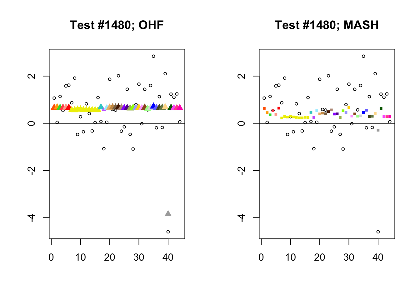
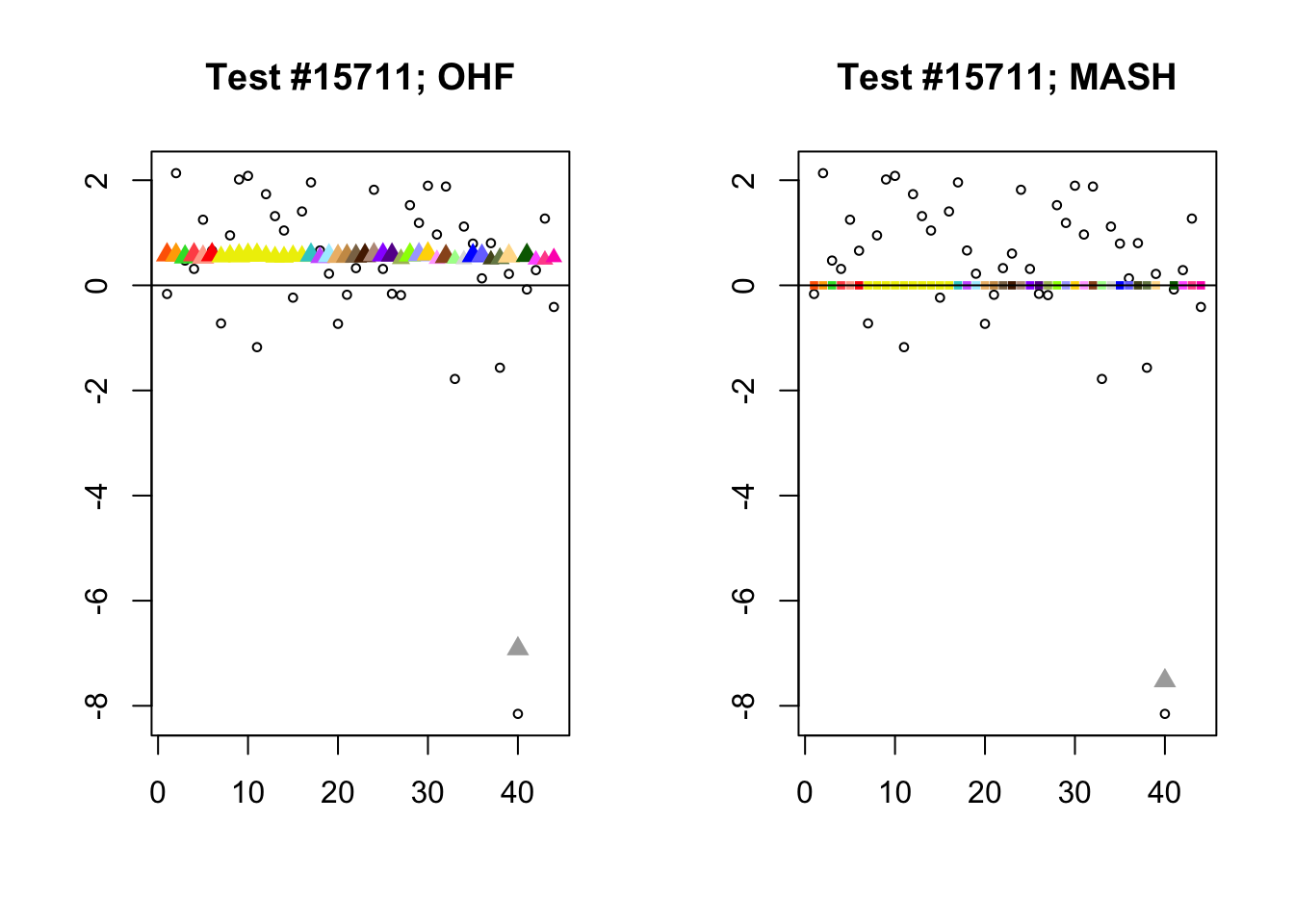
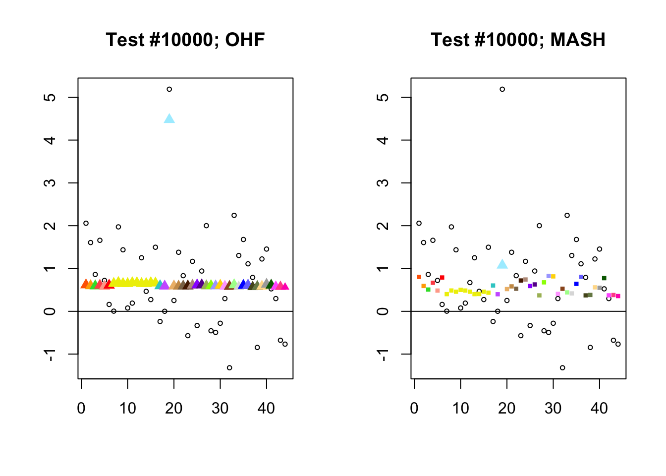
By far the most common case is one in which FLASH finds a combination of a small equal effect and a large unique effect, while MASH only finds the unique effect to be significant. (Here, it is possibly relevant to recall that my simulation study suggested that FLASH outperforms MASH when the “true” effect is a combination of an equal effect and a unique effect.) In such cases, FLASH usually (but not always) applies far less shrinkage to the unique effect. Some typical examples follow.
# interesting.tests <- compare_methods(fl_lfsr, m_lfsr, fl_pm, m_pm)

par(mfrow=c(1, 2))

identical.plus.unique <- c(15828, 1480, 15711, 10000)
for (n in identical.plus.unique) {
  plot_test(n, fl_lfsr, fl_pm, "OHF")
  plot_test(n, m_lfsr, m_pm, "MASH")
}
Expand here to see past versions of ohf_not_mash-1.png:
| Version | Author | Date |
|---|---|---|
| a91ab89 | Jason Willwerscheid | 2018-08-02 |
Expand here to see past versions of ohf_not_mash-2.png:
| Version | Author | Date |
|---|---|---|
| a91ab89 | Jason Willwerscheid | 2018-08-02 |
Expand here to see past versions of ohf_not_mash-3.png:
| Version | Author | Date |
|---|---|---|
| a91ab89 | Jason Willwerscheid | 2018-08-02 |
Expand here to see past versions of ohf_not_mash-4.png:
| Version | Author | Date |
|---|---|---|
| a91ab89 | Jason Willwerscheid | 2018-08-02 |
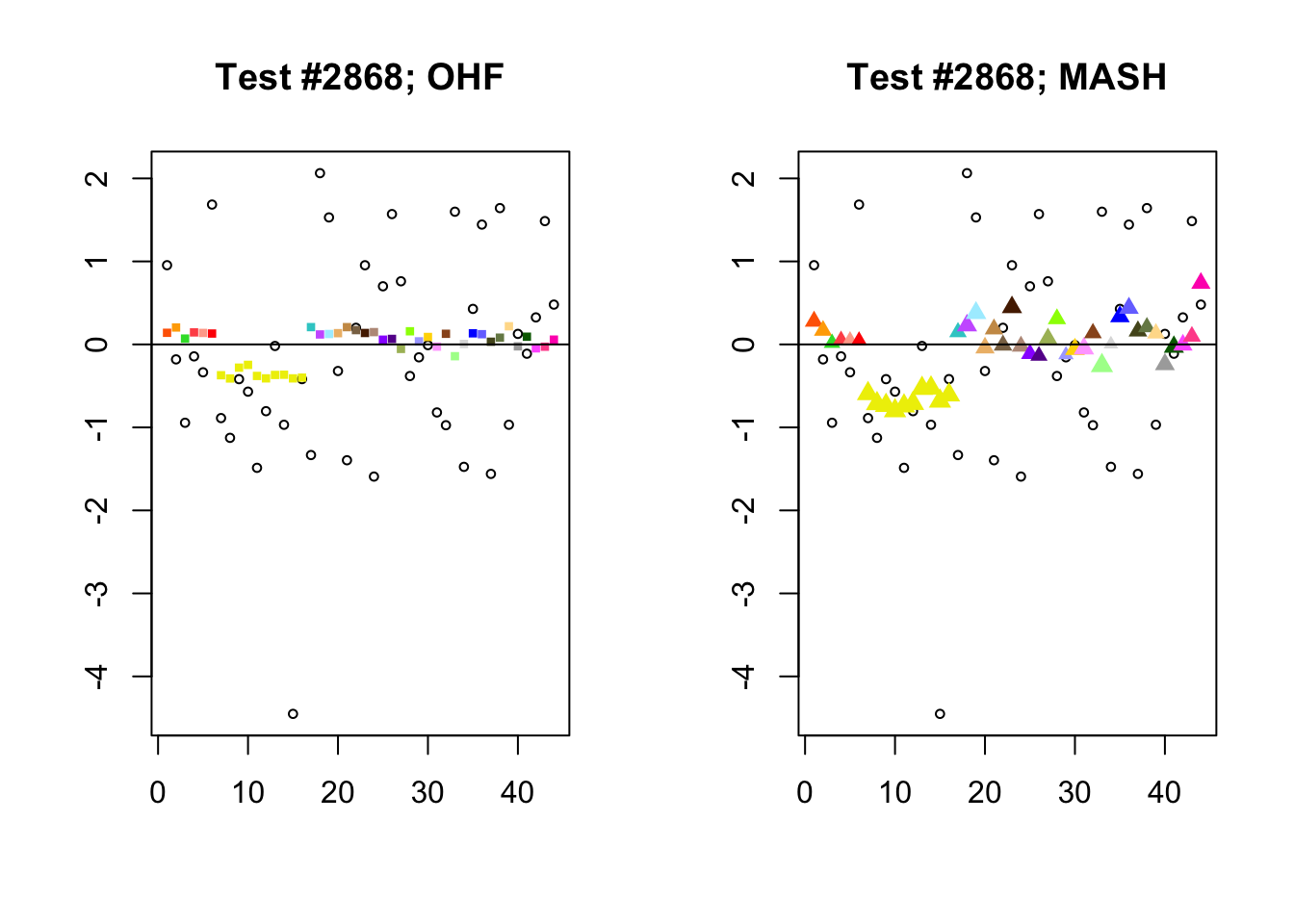
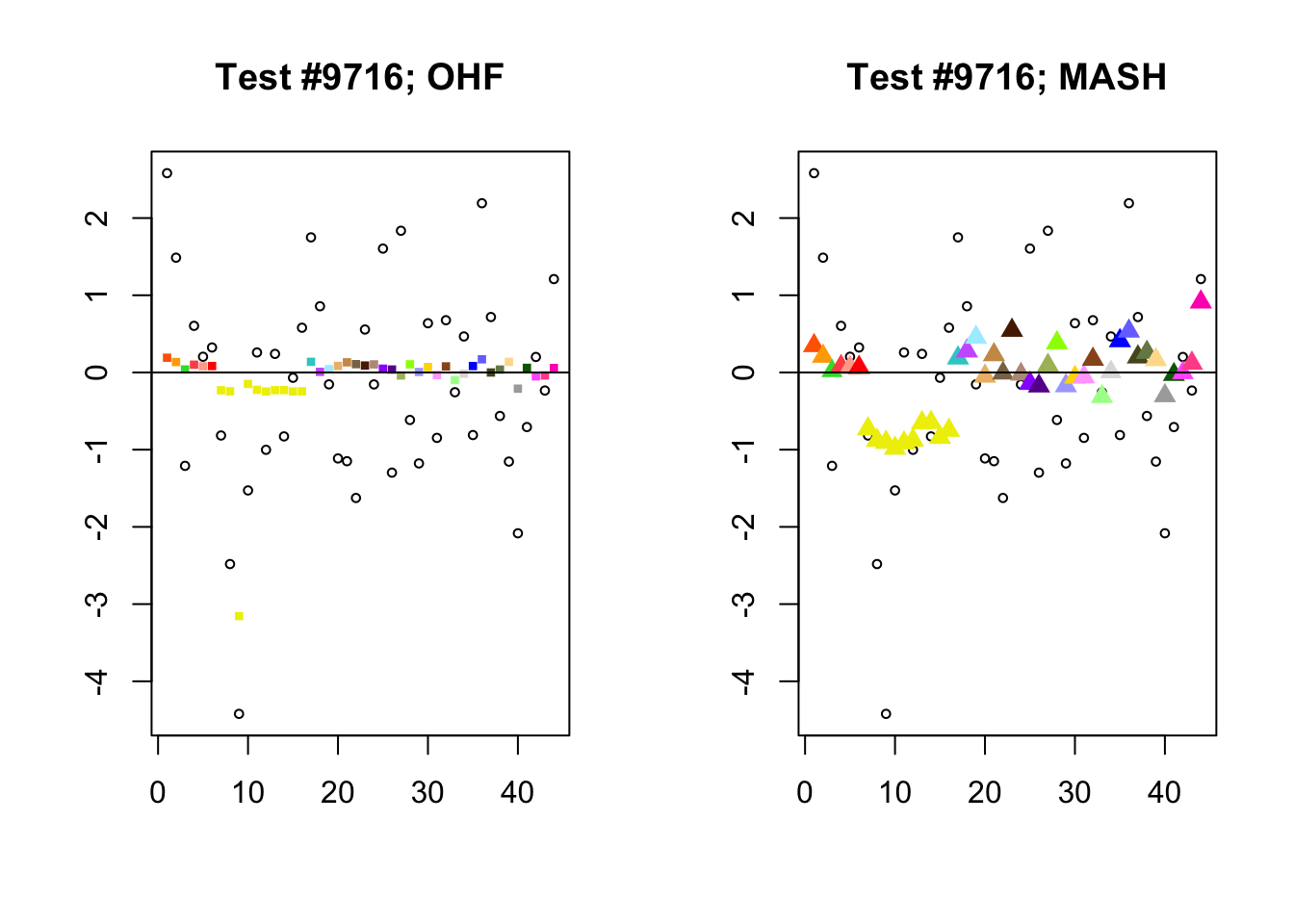
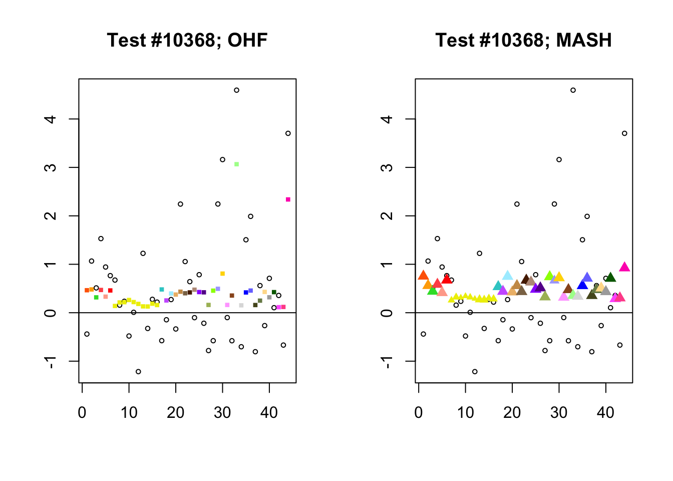
Significant for MASH, not OHF
To understand the typical situation where MASH declares effects to be significant but OHF does not, recall from my analysis of GTEx workflows that the MASH fit puts large mixture weights on data-driven covariance matrices (around 0.6 on “ED_tPCA” and 0.25 on “ED_PCA_2”) and a comparatively small weight (around 0.1) on the “equal effects” covariance structure. In contrast, the equal effects loading accounts for about 70% of the variance explained by the OHF fit. This, I think, is why OHF is so much more likely to find an equal effect in the tests above. MASH, on the contrary, is more likely to find a pattern of covariance that derives from the data-driven structures. Notice the similarity of the MASH estimates in the following tests (in the last example, signs are reversed):
par(mfrow=c(1, 2))

mash.covar <- c(2868, 9716, 10368, 9716)
for (n in mash.covar) {
  plot_test(n, fl_lfsr, fl_pm, "OHF")
  plot_test(n, m_lfsr, m_pm, "MASH")
}
Expand here to see past versions of mash_not_ohf-1.png:
| Version | Author | Date |
|---|---|---|
| a91ab89 | Jason Willwerscheid | 2018-08-02 |
Expand here to see past versions of mash_not_ohf-2.png:
| Version | Author | Date |
|---|---|---|
| a91ab89 | Jason Willwerscheid | 2018-08-02 |
Expand here to see past versions of mash_not_ohf-3.png:
| Version | Author | Date |
|---|---|---|
| a91ab89 | Jason Willwerscheid | 2018-08-02 |

Expand here to see past versions of mash_not_ohf-4.png:
| Version | Author | Date |
|---|---|---|
| a91ab89 | Jason Willwerscheid | 2018-08-02 |
At first, it seems bizarre that effects with posterior means near zero are judged to be significant. My guess is that in each of these cases, the observations follow a pattern that closely matches the data-driven covariance structures, so that MASH can be highly confident in the sign of the effect even if the effect is not very large.
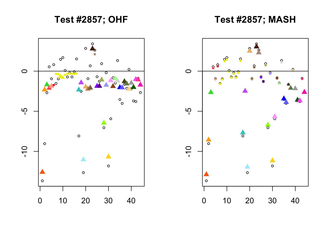
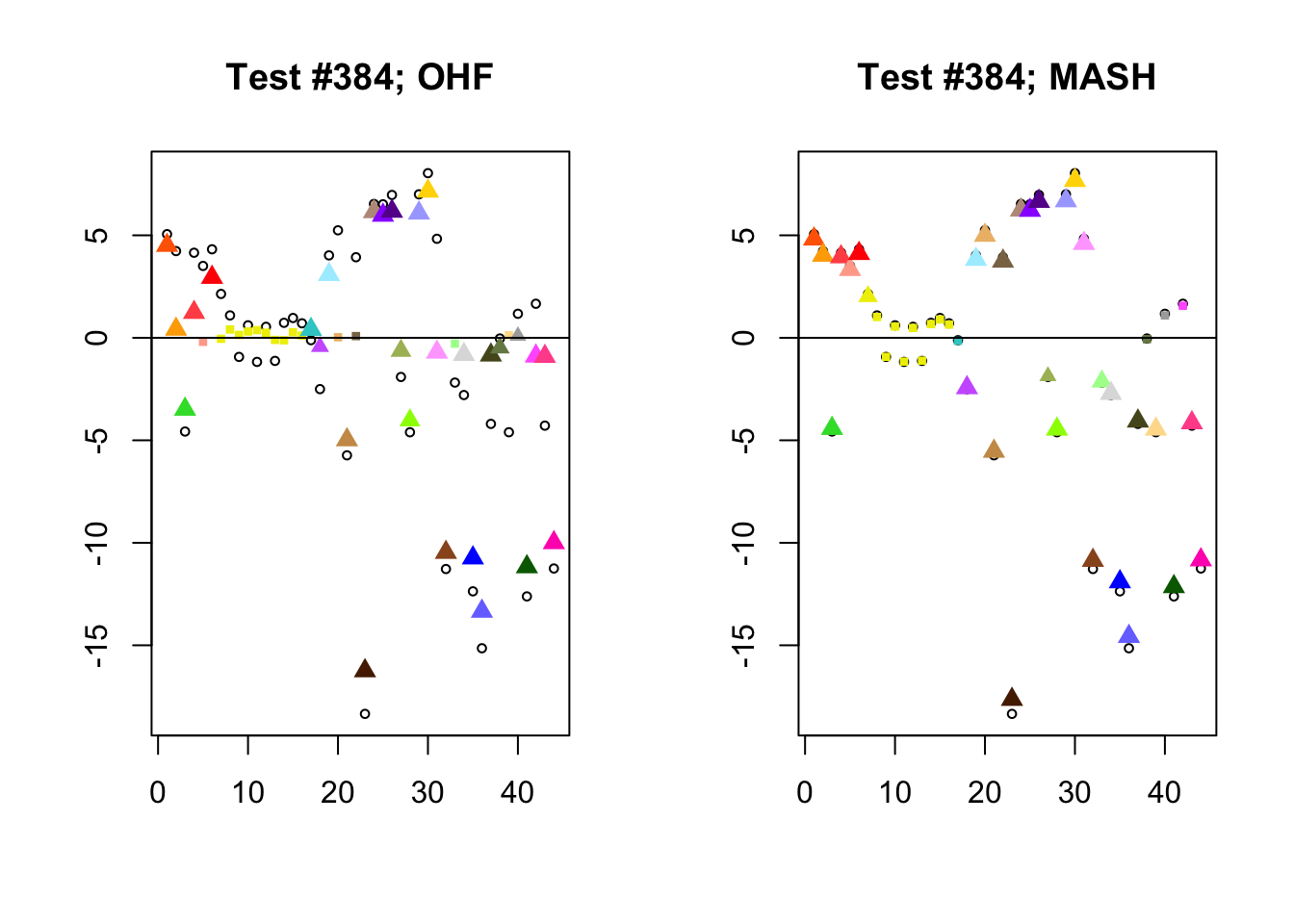
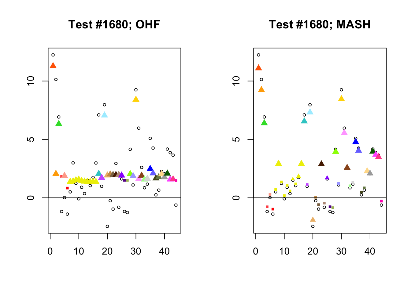
Different posterior means
I conclude with some examples of tests with a large mean squared difference in posterior means. As might be expected, these are all tests where effect sizes are large for many conditions. Interestingly, MASH applies little to no shrinkage in such cases (even for small effects). FLASH does a better job applying a reasonable amount of shrinkage to small and moderate effects, but can be overly aggressive in shrinking large effects.
In test #2857, for example, FLASH applies a huge amount of shrinkage to the large effects observed in visceral adipose omental tissue and in mammary tissue, shrinking the \(z\)-scores from -9.0 to -2.3 and from -8.1 to -2.3, respectively. These are both tissues for which the prior on the unique effect is heavily concentrated near zero (see here), so the results make sense given the FLASH fit, but the shrinkage still seems extreme. I think that this problem could be mitigated by training on a larger subset of random tests (so that some examples of large effects in these tissues get included).
In contrast, the MASH posterior mixture weights for test #2857 are heavily concentrated on the simple_het matrices, which posit only weak correlations among conditions.
par(mfrow=c(1, 2))

diff.pms <- c(2857, 697, 384, 1680)
for (n in diff.pms) {
  plot_test(n, fl_lfsr, fl_pm, "OHF")
  plot_test(n, m_lfsr, m_pm, "MASH")
}
Expand here to see past versions of diff_pms-1.png:
| Version | Author | Date |
|---|---|---|
| ea857fe | Jason Willwerscheid | 2018-08-03 |
Expand here to see past versions of diff_pms-2.png:
| Version | Author | Date |
|---|---|---|
| ea857fe | Jason Willwerscheid | 2018-08-03 |
Expand here to see past versions of diff_pms-3.png:
| Version | Author | Date |
|---|---|---|
| ea857fe | Jason Willwerscheid | 2018-08-03 |
Expand here to see past versions of diff_pms-4.png:
| Version | Author | Date |
|---|---|---|
| ea857fe | Jason Willwerscheid | 2018-08-03 |
Session information
sessionInfo()R version 3.4.3 (2017-11-30)
Platform: x86_64-apple-darwin15.6.0 (64-bit)
Running under: macOS High Sierra 10.13.6
Matrix products: default
BLAS: /Library/Frameworks/R.framework/Versions/3.4/Resources/lib/libRblas.0.dylib
LAPACK: /Library/Frameworks/R.framework/Versions/3.4/Resources/lib/libRlapack.dylib
locale:
[1] en_US.UTF-8/en_US.UTF-8/en_US.UTF-8/C/en_US.UTF-8/en_US.UTF-8
attached base packages:
[1] stats graphics grDevices utils datasets methods base
other attached packages:
[1] flashr_0.5-12 mashr_0.2-7 ashr_2.2-10
loaded via a namespace (and not attached):
[1] Rcpp_0.12.17 pillar_1.2.1 compiler_3.4.3
[4] git2r_0.21.0 plyr_1.8.4 workflowr_1.0.1
[7] R.methodsS3_1.7.1 R.utils_2.6.0 iterators_1.0.9
[10] tools_3.4.3 testthat_2.0.0 digest_0.6.15
[13] tibble_1.4.2 gtable_0.2.0 evaluate_0.10.1
[16] memoise_1.1.0 lattice_0.20-35 rlang_0.2.0
[19] Matrix_1.2-12 foreach_1.4.4 commonmark_1.4
[22] yaml_2.1.17 parallel_3.4.3 ebnm_0.1-12
[25] mvtnorm_1.0-7 xml2_1.2.0 withr_2.1.1.9000
[28] stringr_1.3.0 knitr_1.20 roxygen2_6.0.1.9000
[31] devtools_1.13.4 rprojroot_1.3-2 grid_3.4.3
[34] R6_2.2.2 rmarkdown_1.8 rmeta_3.0
[37] ggplot2_2.2.1 magrittr_1.5 whisker_0.3-2
[40] scales_0.5.0 backports_1.1.2 codetools_0.2-15
[43] htmltools_0.3.6 MASS_7.3-48 assertthat_0.2.0
[46] softImpute_1.4 colorspace_1.3-2 stringi_1.1.6
[49] lazyeval_0.2.1 munsell_0.4.3 doParallel_1.0.11
[52] pscl_1.5.2 truncnorm_1.0-8 SQUAREM_2017.10-1
[55] R.oo_1.21.0 This reproducible R Markdown analysis was created with workflowr 1.0.1