MASH v FLASH GTEx analysis: MASH v “Top 20”
Last updated: 2018-08-04
workflowr checks: (Click a bullet for more information)-
✔ R Markdown file: up-to-date
Great! Since the R Markdown file has been committed to the Git repository, you know the exact version of the code that produced these results.
-
✔ Environment: empty
Great job! The global environment was empty. Objects defined in the global environment can affect the analysis in your R Markdown file in unknown ways. For reproduciblity it’s best to always run the code in an empty environment.
-
✔ Seed:
set.seed(20180609)The command
set.seed(20180609)was run prior to running the code in the R Markdown file. Setting a seed ensures that any results that rely on randomness, e.g. subsampling or permutations, are reproducible. -
✔ Session information: recorded
Great job! Recording the operating system, R version, and package versions is critical for reproducibility.
-
Great! You are using Git for version control. Tracking code development and connecting the code version to the results is critical for reproducibility. The version displayed above was the version of the Git repository at the time these results were generated.✔ Repository version: 312476b
Note that you need to be careful to ensure that all relevant files for the analysis have been committed to Git prior to generating the results (you can usewflow_publishorwflow_git_commit). workflowr only checks the R Markdown file, but you know if there are other scripts or data files that it depends on. Below is the status of the Git repository when the results were generated:
Note that any generated files, e.g. HTML, png, CSS, etc., are not included in this status report because it is ok for generated content to have uncommitted changes.Ignored files: Ignored: .DS_Store Ignored: .Rhistory Ignored: .Rproj.user/ Ignored: data/ Ignored: docs/.DS_Store Ignored: docs/images/.DS_Store Ignored: docs/images/.Rapp.history Ignored: output/.DS_Store Ignored: output/.Rapp.history Ignored: output/MASHvFLASHgtex/.DS_Store Ignored: output/MASHvFLASHsims/.DS_Store Ignored: output/MASHvFLASHsims/backfit/.DS_Store Ignored: output/MASHvFLASHsims/backfit/.Rapp.history Untracked files: Untracked: docs/figure/OHFvTop20.Rmd/ Unstaged changes: Modified: code/gtexanalysis.R
Expand here to see past versions:
| File | Version | Author | Date | Message |
|---|---|---|---|---|
| html | 5401954 | Jason Willwerscheid | 2018-08-04 | Build site. |
| Rmd | b2aa853 | Jason Willwerscheid | 2018-08-04 | wflow_publish(c(“analysis/MASHvTop20.Rmd”, |
| html | 592a427 | Jason Willwerscheid | 2018-08-03 | Build site. |
| Rmd | 0d2b9b5 | Jason Willwerscheid | 2018-08-03 | wflow_publish(c(“analysis/index.Rmd”, “analysis/MASHvTop20.Rmd”)) |
| html | 9867668 | Jason Willwerscheid | 2018-08-03 | Build site. |
| Rmd | 5f31e16 | Jason Willwerscheid | 2018-08-03 | wflow_publish(c(“analysis/index.Rmd”, “analysis/MASHvTop20.Rmd”)) |
Introduction
This analysis compares the MASH fit to the “Top 20” fit. See here for fitting details and here for an introduction to the plots.
library(mashr)Loading required package: ashrdevtools::load_all("/Users/willwerscheid/GitHub/flashr/")Loading flashrgtex <- readRDS(gzcon(url("https://github.com/stephenslab/gtexresults/blob/master/data/MatrixEQTLSumStats.Portable.Z.rds?raw=TRUE")))
strong <- t(gtex$strong.z)
fpath <- "./output/MASHvFLASHgtex2/"
m_final <- readRDS(paste0(fpath, "m.rds"))
fl_final <- readRDS(paste0(fpath, "Top20.rds"))
m_lfsr <- t(get_lfsr(m_final))
m_pm <- t(get_pm(m_final))
all_fl_lfsr <- readRDS(paste0(fpath, "fllfsr.rds"))
fl_lfsr <- all_fl_lfsr[[4]]
fl_pm <- flash_get_fitted_values(fl_final)missing.tissues <- c(7, 8, 19, 20, 24, 25, 31, 34, 37)
gtex.colors <- read.table("https://github.com/stephenslab/gtexresults/blob/master/data/GTExColors.txt?raw=TRUE", sep = '\t', comment.char = '')[-missing.tissues, 2]
OHF.colors <- c("tan4", "tan3")
zero.colors <- c("black", gray.colors(19, 0.2, 0.9),
gray.colors(17, 0.95, 1))
plot_test <- function(n, lfsr, pm, method_name) {
plot(strong[, n], pch=1, col="black", xlab="", ylab="", cex=0.6,
ylim=c(min(c(strong[, n], 0)), max(c(strong[, n], 0))),
main=paste0("Test #", n, "; ", method_name))
size = rep(0.6, 44)
shape = rep(15, 44)
signif <- lfsr[, n] <= .05
shape[signif] <- 17
size[signif] <- 1.35 - 15 * lfsr[signif, n]
size <- pmin(size, 1.2)
points(pm[, n], pch=shape, col=as.character(gtex.colors), cex=size)
abline(0, 0)
}
plot_ohf_v_ohl_loadings <- function(n, ohf_fit, ohl_fit, ohl_name,
legend_pos = "bottomright") {
ohf <- abs(ohf_fit$EF[n, ] * apply(abs(ohf_fit$EL), 2, max))
ohl <- -abs(ohl_fit$EF[n, ] * apply(abs(ohl_fit$EL), 2, max))
data <- rbind(c(ohf, rep(0, length(ohl) - 45)),
c(ohl[1:45], rep(0, length(ohf) - 45),
ohl[46:length(ohl)]))
colors <- c("black",
as.character(gtex.colors),
OHF.colors,
zero.colors[1:(length(ohl) - 45)])
x <- barplot(data, beside=T, col=rep(colors, each=2),
main=paste0("Test #", n, " loadings"),
legend.text = c("OHF", ohl_name),
args.legend = list(x = legend_pos, bty = "n", pch="+-",
fill=NULL, border="white"))
text(x[2*(46:47) - 1], min(data) / 10,
labels=as.character(1:2), cex=0.4)
text(x[2*(48:ncol(data))], max(data) / 10,
labels=as.character(1:(length(ohl) - 45)), cex=0.4)
}
compare_methods <- function(lfsr1, lfsr2, pm1, pm2) {
res <- list()
res$first_not_second <- find_A_not_B(lfsr1, lfsr2)
res$lg_first_not_second <- find_large_A_not_B(lfsr1, lfsr2)
res$second_not_first <- find_A_not_B(lfsr2, lfsr1)
res$lg_second_not_first <- find_large_A_not_B(lfsr2, lfsr1)
res$diff_pms <- find_overall_pm_diff(pm1, pm2)
return(res)
}
# Find tests where many conditions are significant according to
# method A but not according to method B.
find_A_not_B <- function(lfsrA, lfsrB) {
select_tests(colSums(lfsrA <= 0.05 & lfsrB > 0.05))
}
# Find tests where many conditions are highly significant according to
# method A but are not significant according to method B.
find_large_A_not_B <- function(lfsrA, lfsrB) {
select_tests(colSums(lfsrA <= 0.01 & lfsrB > 0.05))
}
find_overall_pm_diff <- function(pmA, pmB, n = 4) {
pm_diff <- colSums((pmA - pmB)^2)
return(order(pm_diff, decreasing = TRUE)[1:4])
}
# Get at least four (or min_n) "top" tests.
select_tests <- function(colsums, min_n = 4) {
n <- 45
n_tests <- 0
while (n_tests < min_n && n > 0) {
n <- n - 1
n_tests <- sum(colsums >= n)
}
return(which(colsums >= n))
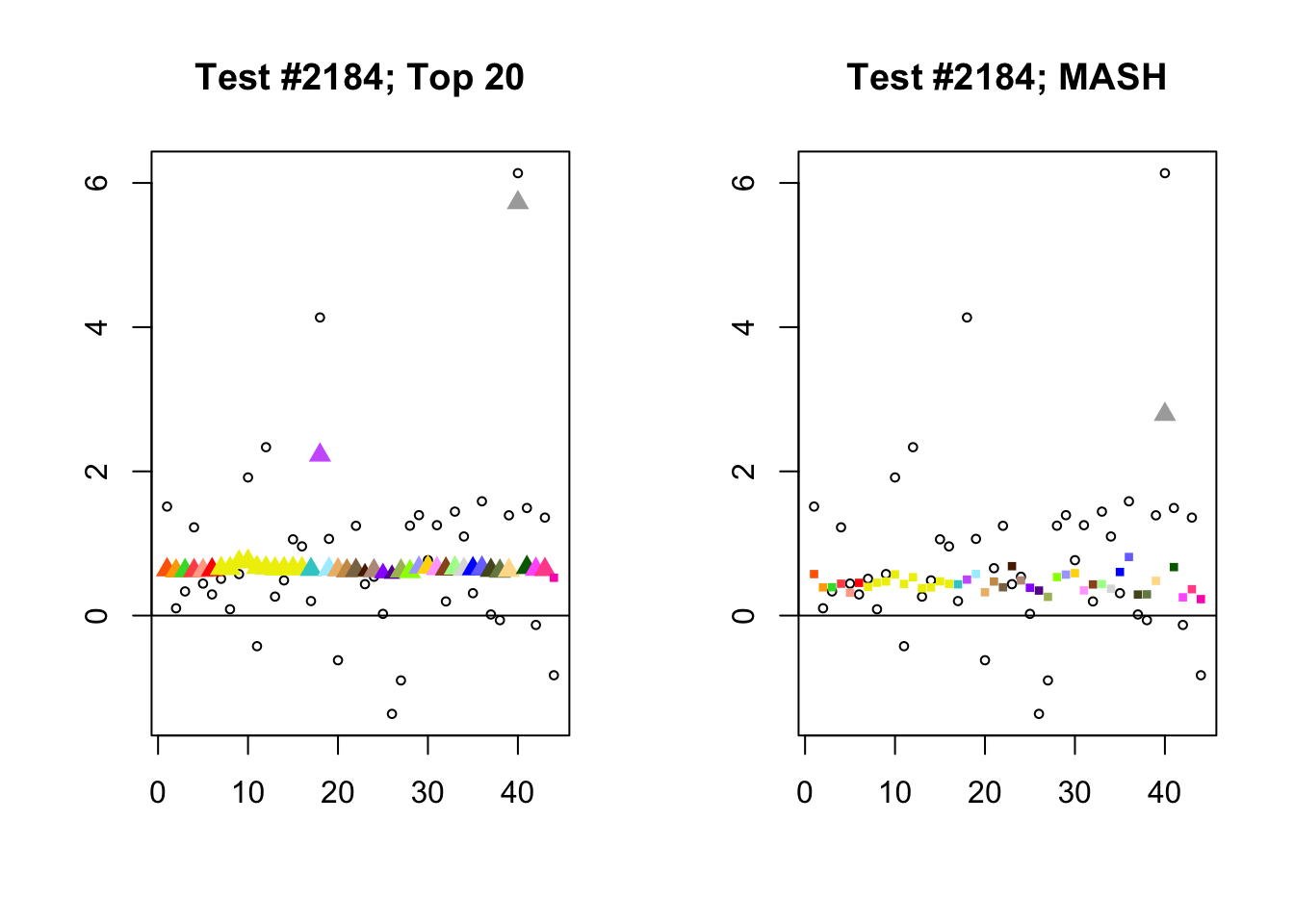
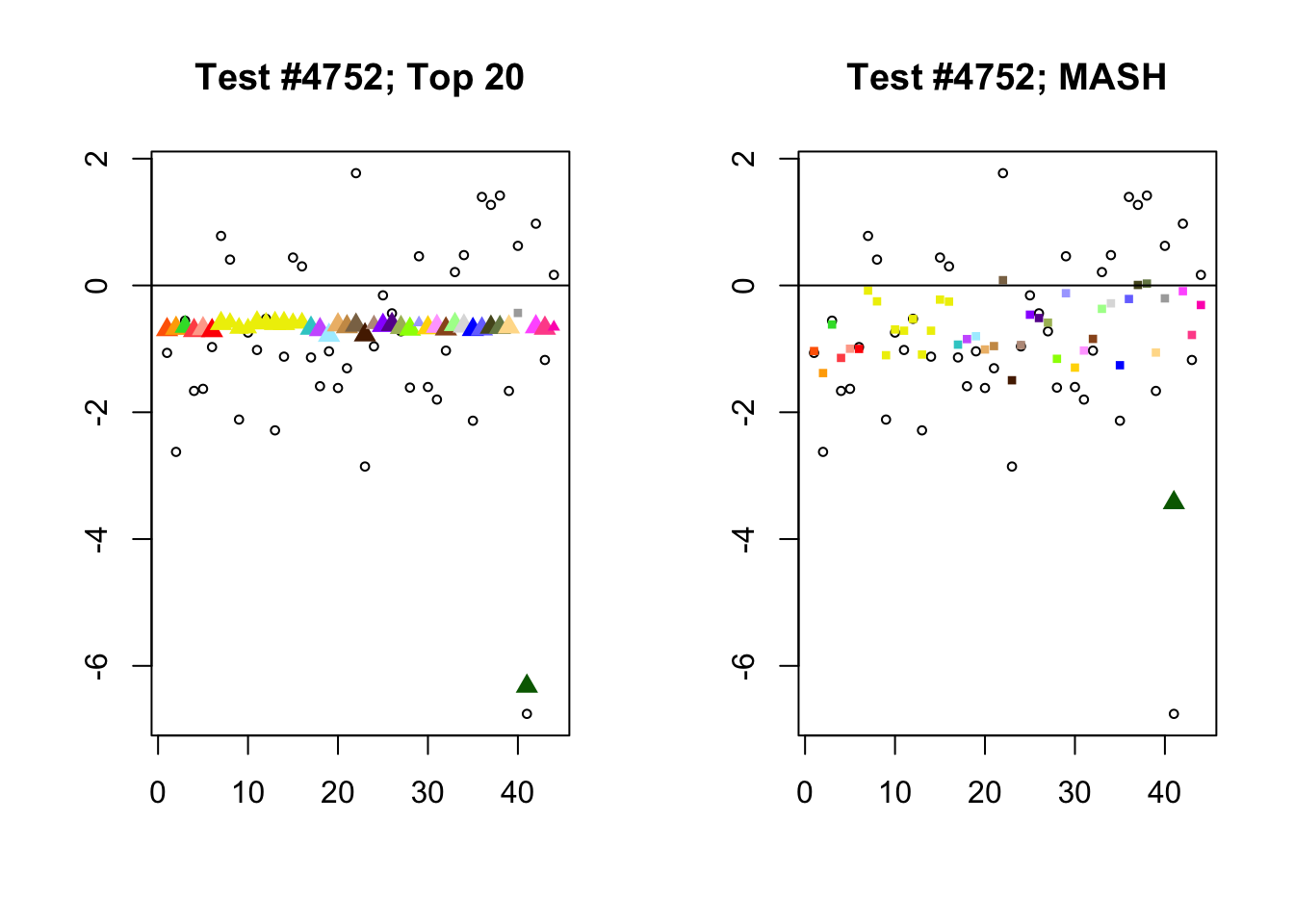
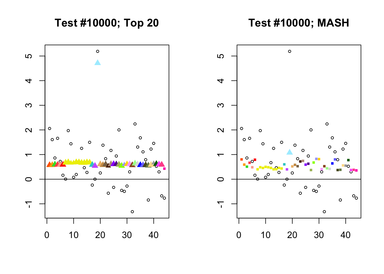
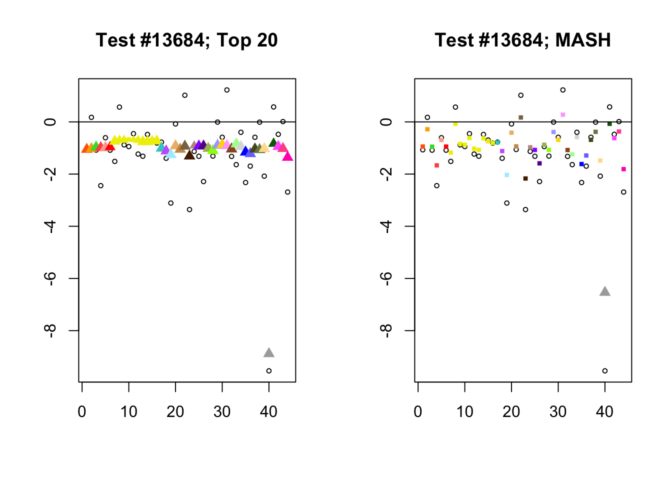
}Significant for Top 20, not MASH
As in the previous analysis, the most common case involves a combination of a small equal effect and a large unique effect. Some typical examples follow.
# mash.v.top20 <- compare_methods(fl_lfsr, m_lfsr, fl_pm, m_pm)

identical.plus.unique <- c(2184, 4752, 10000, 13684)

par(mfrow=c(1, 2))
for (n in identical.plus.unique) {
  plot_test(n, fl_lfsr, fl_pm, "Top 20")
  plot_test(n, m_lfsr, m_pm, "MASH")
}
Expand here to see past versions of ohf_not_mash-1.png:
| Version | Author | Date |
|---|---|---|
| 9867668 | Jason Willwerscheid | 2018-08-03 |
Expand here to see past versions of ohf_not_mash-2.png:
| Version | Author | Date |
|---|---|---|
| 9867668 | Jason Willwerscheid | 2018-08-03 |
Expand here to see past versions of ohf_not_mash-3.png:
| Version | Author | Date |
|---|---|---|
| 9867668 | Jason Willwerscheid | 2018-08-03 |
Expand here to see past versions of ohf_not_mash-4.png:
| Version | Author | Date |
|---|---|---|
| 9867668 | Jason Willwerscheid | 2018-08-03 |
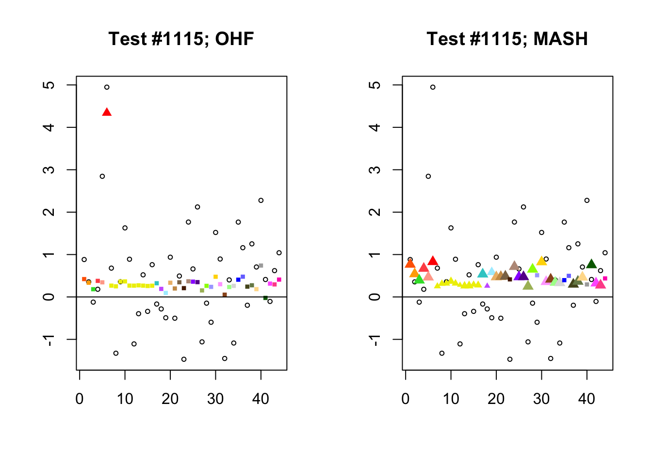
Significant for MASH, not OHF
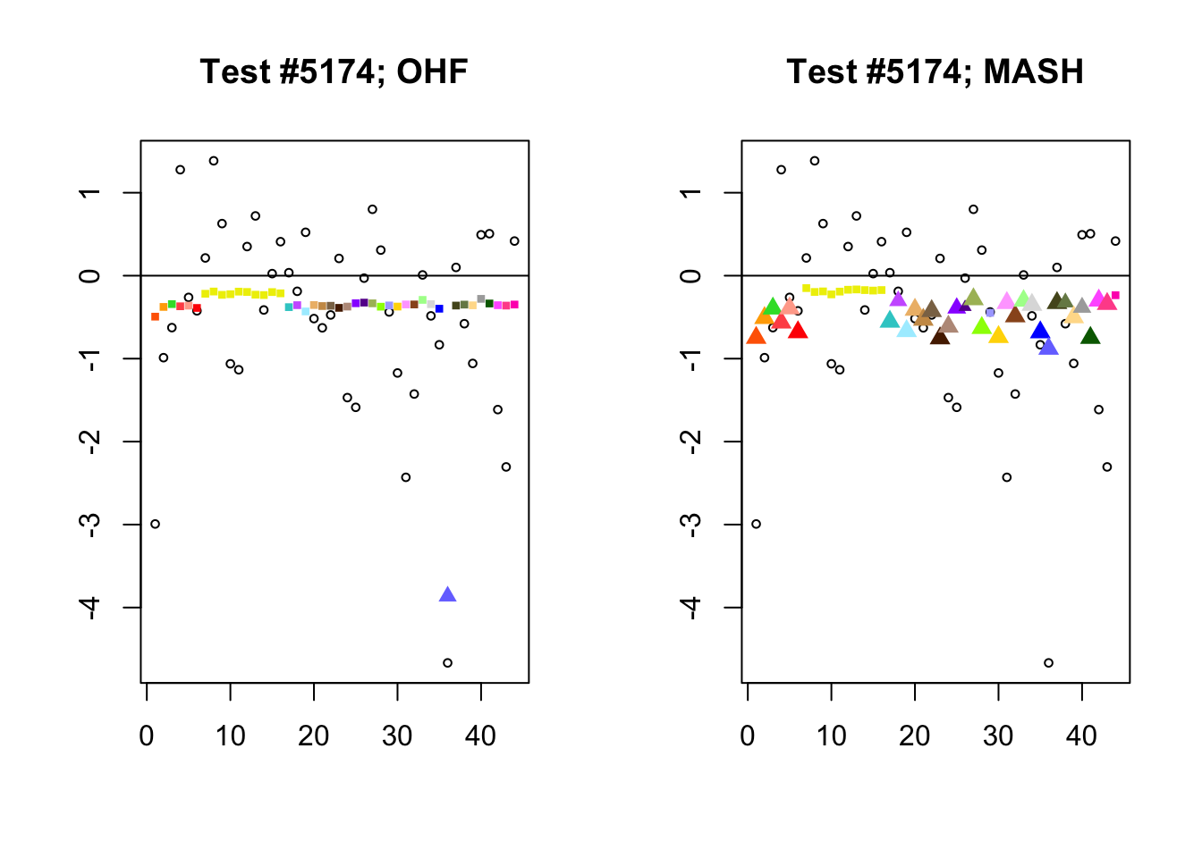
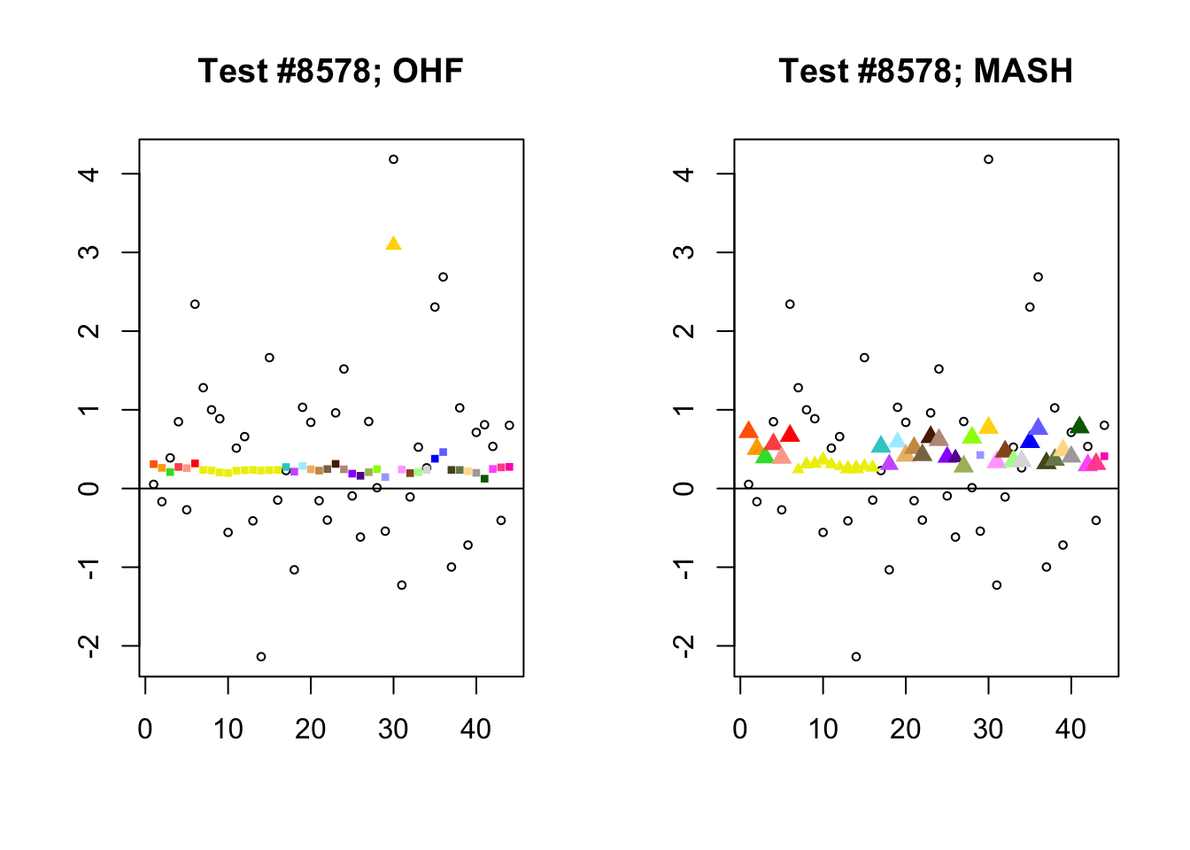
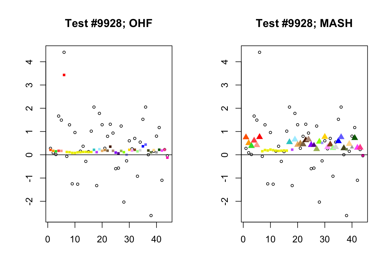
The most typical case here has MASH finding a significant equal effect, while FLASH finds a significant unique effect and an insignificant equal effect. In each of the following tests, there is a single outlying effect (with a raw \(z\)-score of around 4 or 5), which FLASH identifies as unique but which MASH “assigns” to the equal effect (or rather, to the data-driven covariance structure described in the previous analysis). Roughly, the other observations borrow strength from the outlying observation in MASH but not in FLASH.
par(mfrow=c(1, 2))

shrink.unique <- c(1115, 5174, 8578, 9928)

for (n in shrink.unique) {
  plot_test(n, fl_lfsr, fl_pm, "OHF")
  plot_test(n, m_lfsr, m_pm, "MASH")
}
Expand here to see past versions of mash_not_ohf-1.png:
| Version | Author | Date |
|---|---|---|
| 9867668 | Jason Willwerscheid | 2018-08-03 |
Expand here to see past versions of mash_not_ohf-2.png:
| Version | Author | Date |
|---|---|---|
| 9867668 | Jason Willwerscheid | 2018-08-03 |
Expand here to see past versions of mash_not_ohf-3.png:
| Version | Author | Date |
|---|---|---|
| 9867668 | Jason Willwerscheid | 2018-08-03 |
Expand here to see past versions of mash_not_ohf-4.png:
| Version | Author | Date |
|---|---|---|
| 9867668 | Jason Willwerscheid | 2018-08-03 |
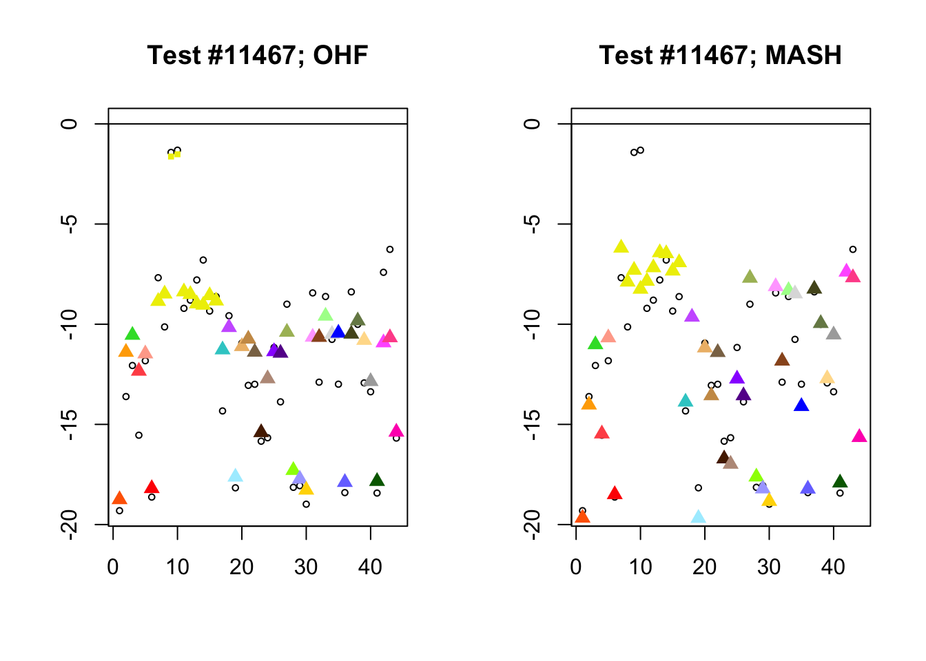
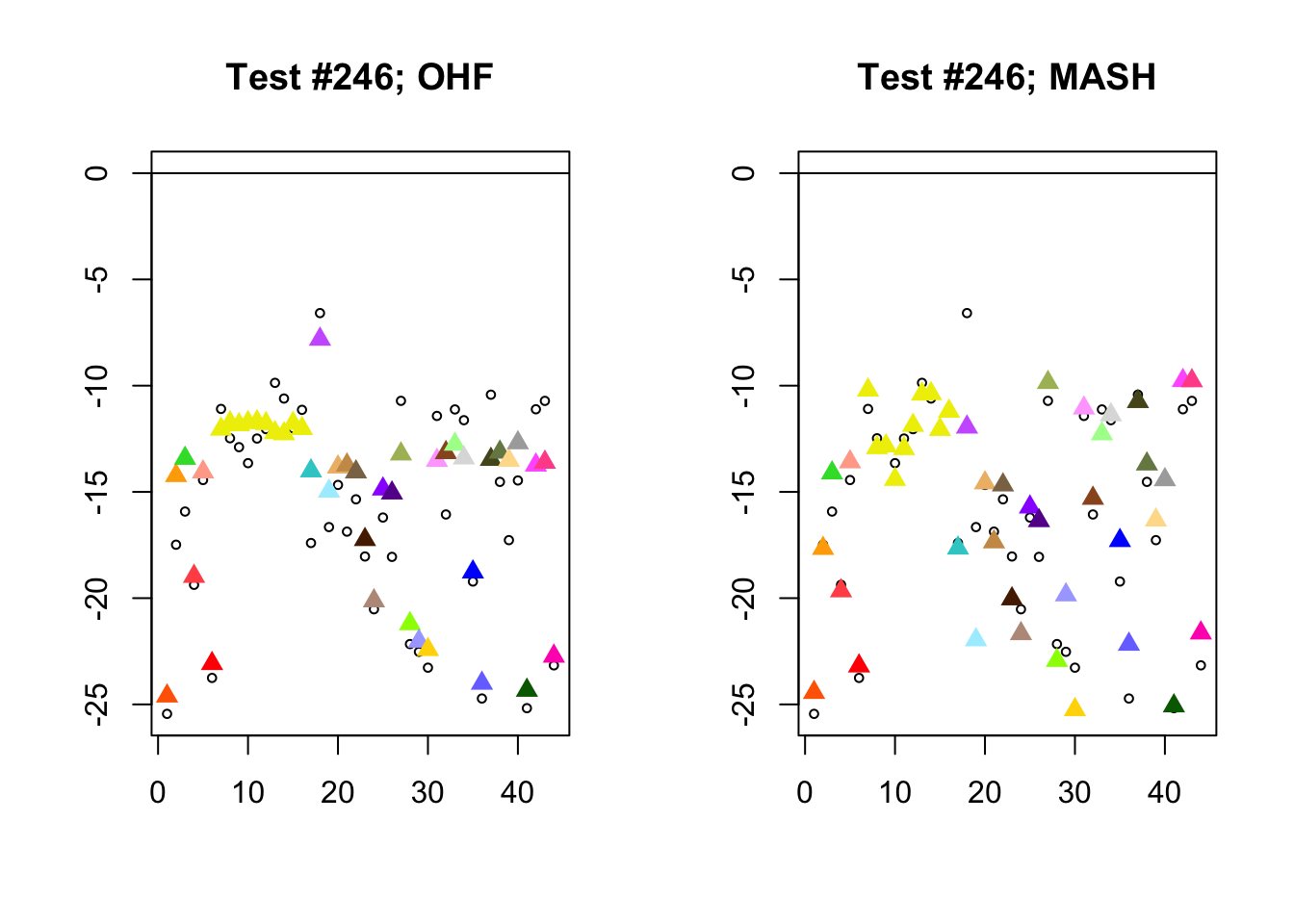
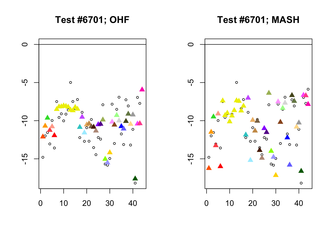
Different posterior means
The following examples differ from the examples in the previous analysis in that all effect sizes are large. As a result, the MASH estimates do not coincide with the raw observations as neatly. Notice, for example, that in each case some of the MASH estimates are even larger than the observed effect sizes. This is because the posterior mixture weights are primarily concentrated on the ED_tPCA matrices rather than on the simple_het matrices (see here for a description of these matrices).
par(mfrow=c(1, 2))

diff.pms <- c(11467, 246, 6701)
for (n in diff.pms) {
  plot_test(n, fl_lfsr, fl_pm, "OHF")
  plot_test(n, m_lfsr, m_pm, "MASH")
}
Expand here to see past versions of diff_pms-1.png:
| Version | Author | Date |
|---|---|---|
| 5401954 | Jason Willwerscheid | 2018-08-04 |
Expand here to see past versions of diff_pms-2.png:
| Version | Author | Date |
|---|---|---|
| 5401954 | Jason Willwerscheid | 2018-08-04 |
Expand here to see past versions of diff_pms-3.png:
| Version | Author | Date |
|---|---|---|
| 5401954 | Jason Willwerscheid | 2018-08-04 |
Session information
sessionInfo()R version 3.4.3 (2017-11-30)
Platform: x86_64-apple-darwin15.6.0 (64-bit)
Running under: macOS High Sierra 10.13.6
Matrix products: default
BLAS: /Library/Frameworks/R.framework/Versions/3.4/Resources/lib/libRblas.0.dylib
LAPACK: /Library/Frameworks/R.framework/Versions/3.4/Resources/lib/libRlapack.dylib
locale:
[1] en_US.UTF-8/en_US.UTF-8/en_US.UTF-8/C/en_US.UTF-8/en_US.UTF-8
attached base packages:
[1] stats graphics grDevices utils datasets methods base
other attached packages:
[1] flashr_0.5-12 mashr_0.2-7 ashr_2.2-10
loaded via a namespace (and not attached):
[1] Rcpp_0.12.17 pillar_1.2.1 compiler_3.4.3
[4] git2r_0.21.0 plyr_1.8.4 workflowr_1.0.1
[7] R.methodsS3_1.7.1 R.utils_2.6.0 iterators_1.0.9
[10] tools_3.4.3 testthat_2.0.0 digest_0.6.15
[13] tibble_1.4.2 gtable_0.2.0 evaluate_0.10.1
[16] memoise_1.1.0 lattice_0.20-35 rlang_0.2.0
[19] Matrix_1.2-12 foreach_1.4.4 commonmark_1.4
[22] yaml_2.1.17 parallel_3.4.3 ebnm_0.1-12
[25] mvtnorm_1.0-7 xml2_1.2.0 withr_2.1.1.9000
[28] stringr_1.3.0 knitr_1.20 roxygen2_6.0.1.9000
[31] devtools_1.13.4 rprojroot_1.3-2 grid_3.4.3
[34] R6_2.2.2 rmarkdown_1.8 rmeta_3.0
[37] ggplot2_2.2.1 magrittr_1.5 whisker_0.3-2
[40] scales_0.5.0 backports_1.1.2 codetools_0.2-15
[43] htmltools_0.3.6 MASS_7.3-48 assertthat_0.2.0
[46] softImpute_1.4 colorspace_1.3-2 stringi_1.1.6
[49] lazyeval_0.2.1 munsell_0.4.3 doParallel_1.0.11
[52] pscl_1.5.2 truncnorm_1.0-8 SQUAREM_2017.10-1
[55] R.oo_1.21.0 This reproducible R Markdown analysis was created with workflowr 1.0.1