MASH v FLASH GTEx analysis: nonnegative loadings

Introduction

Here I fit MASH and FLASH objects to the “strong” GTEx dataset using the nonnegative loadings obtained in the previous analysis. See below for code and here for an introduction to the plots below.

Fitting methods

The workflows are similar to those described here.

The workflow for FLASH is identical, except that I use the nonnegative loadings from the previous analysis as my “data-driven” loadings. (To save time, I only use the loadings corresponding to “multi-tissue effects,” since the other loadings are well represented by “canonical” loadings. Further, to aid interpretation, I normalize the loadings so that each has \(\ell_\infty\)-norm equal to 1.)

The workflow for MASH is also identical, except that I use rank-one matrices derived from the nonnegative loadings rather than rank-one matrices obtained using Extreme Deconvolution. More precisely, for each multi-tissue effect \(\ell_i\), I add the matrix \(\ell_i \ell_i^T\) to the list of matrices \(U_i\) in the MASH mixture model.

Results

I pre-run the code and load the fits from file.

library(mashr)

Loading required package: ashr

devtools::load_all("/Users/willwerscheid/GitHub/flashr/")

Loading flashr

source("./code/gtexanalysis.R")

gtex <- readRDS(gzcon(url("https://github.com/stephenslab/gtexresults/blob/master/data/MatrixEQTLSumStats.Portable.Z.rds?raw=TRUE")))
strong <- t(gtex$strong.z)

fpath <- "./output/MASHvFLASHgtex3/"
m_final <- readRDS(paste0(fpath, "m.rds"))
fl_final <- readRDS(paste0(fpath, "fl.rds"))

m_lfsr <- t(get_lfsr(m_final))
m_pm <- t(get_pm(m_final))

fl_lfsr <- readRDS(paste0(fpath, "fllfsr.rds"))
fl_pm <- flash_get_fitted_values(fl_final)

There is significant disagreement between the two fits:

signif_by_mash = as.vector(m_lfsr < 0.05)
signif_by_flash = as.vector(fl_lfsr < 0.05)

round(table(signif_by_mash, signif_by_flash) / length(signif_by_mash),
      digits = 2)

              signif_by_flash
signif_by_mash FALSE TRUE
         FALSE  0.31 0.17
         TRUE   0.08 0.44

Significant for FLASH, not MASH

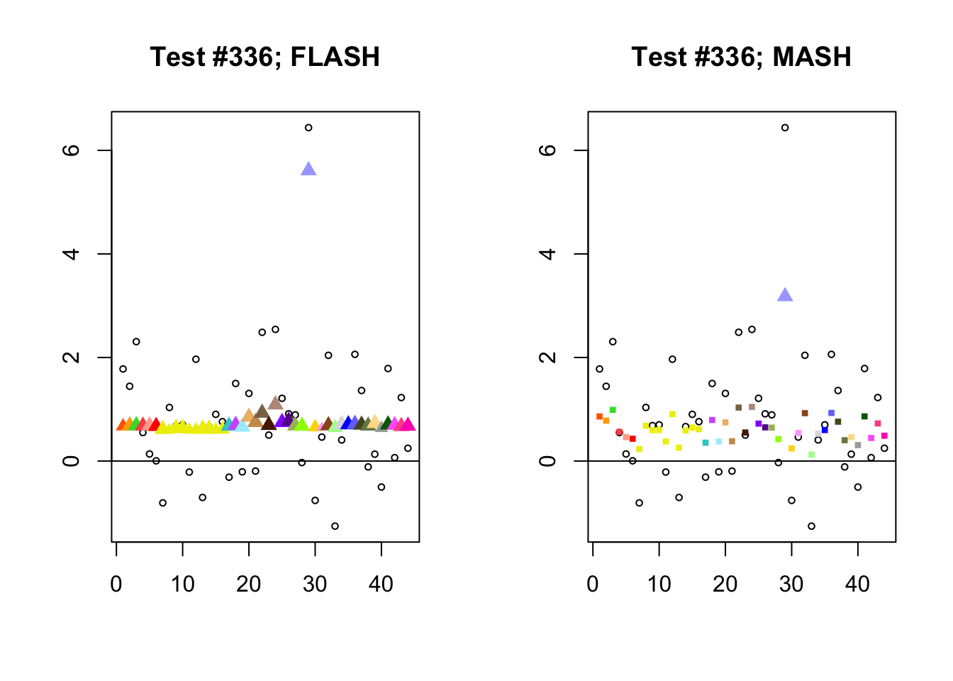
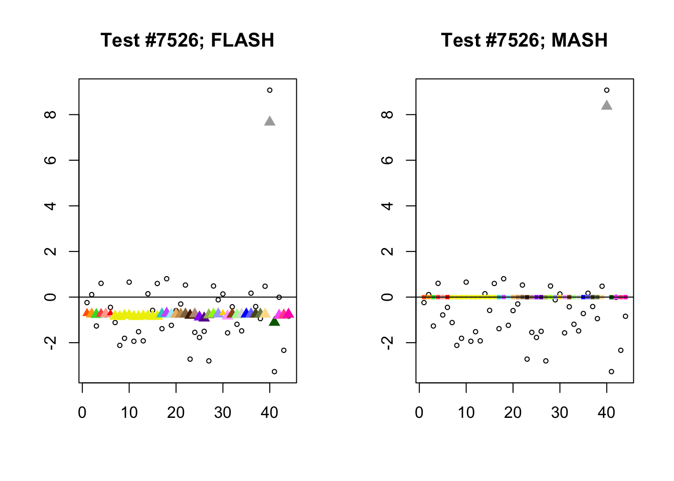
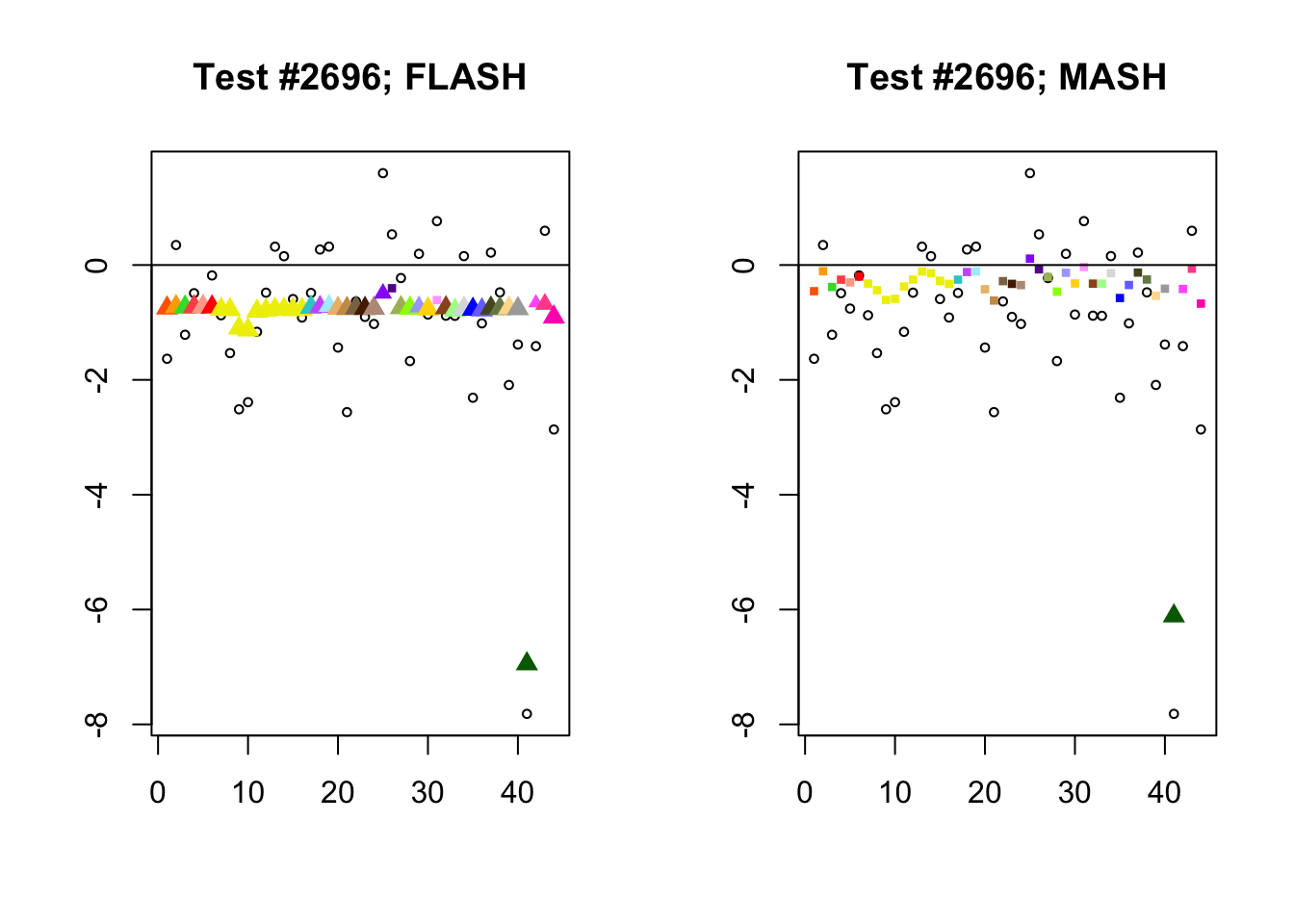
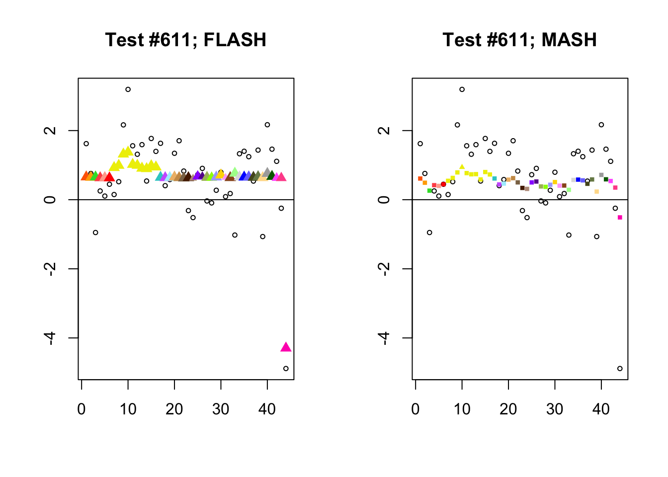
As discussed in previous analyses (see, for example, here), FLASH often finds a combination of a large unique effect and a small equal effect where MASH only finds the unique effect to be significant (or, more rarely, no effects).

# interesting.tests <- compare_methods(fl_lfsr, m_lfsr, fl_pm, m_pm)

par(mfrow=c(1, 2))

identical.plus.unique <- c(336, 7526, 2696, 611)
for (n in identical.plus.unique) {
  plot_test(n, fl_lfsr, fl_pm, "FLASH")
  plot_test(n, m_lfsr, m_pm, "MASH")
}

Expand here to see past versions of flash_not_mash-1.png:

Version	Author	Date
48615e4	Jason Willwerscheid	2018-08-15

Expand here to see past versions of flash_not_mash-2.png:

Version	Author	Date
48615e4	Jason Willwerscheid	2018-08-15

Expand here to see past versions of flash_not_mash-3.png:

Version	Author	Date
48615e4	Jason Willwerscheid	2018-08-15

Expand here to see past versions of flash_not_mash-4.png:

Version	Author	Date
48615e4	Jason Willwerscheid	2018-08-15

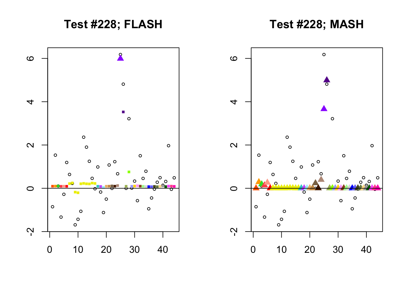
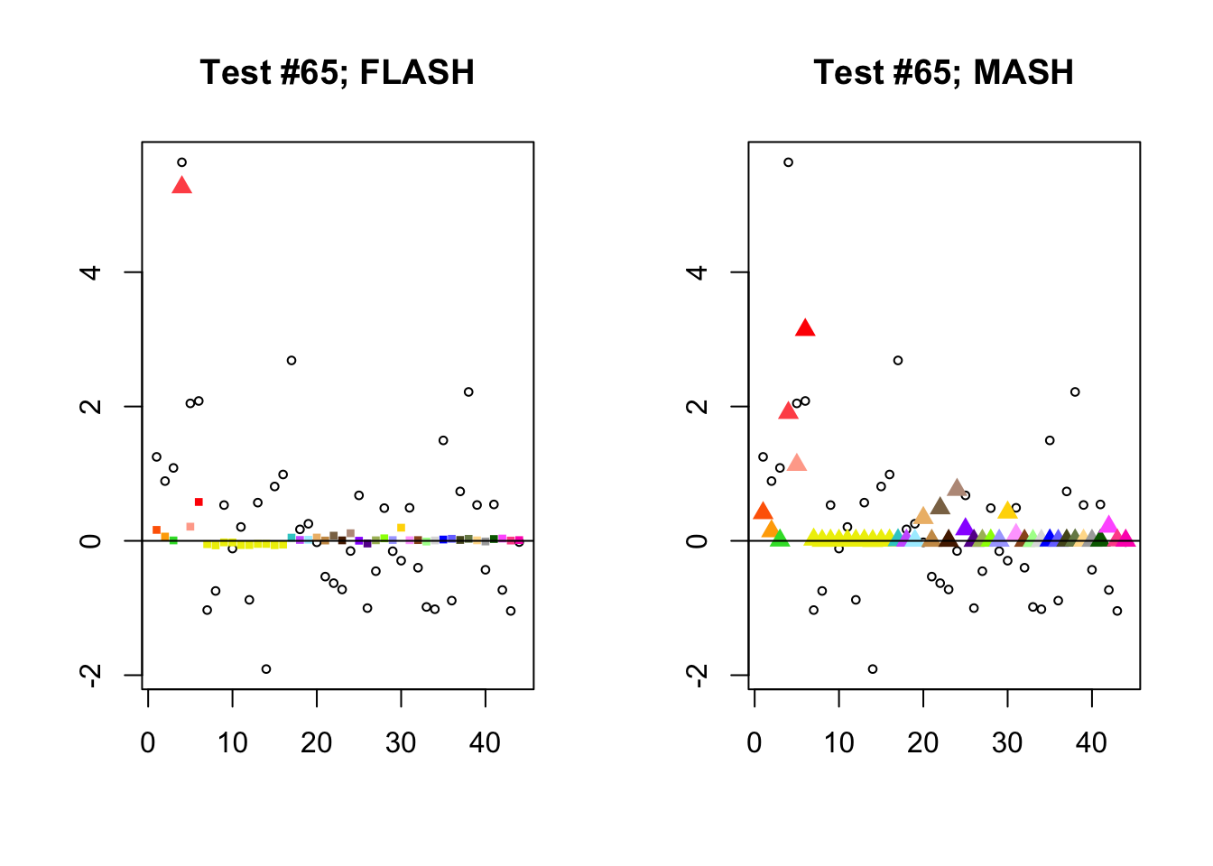
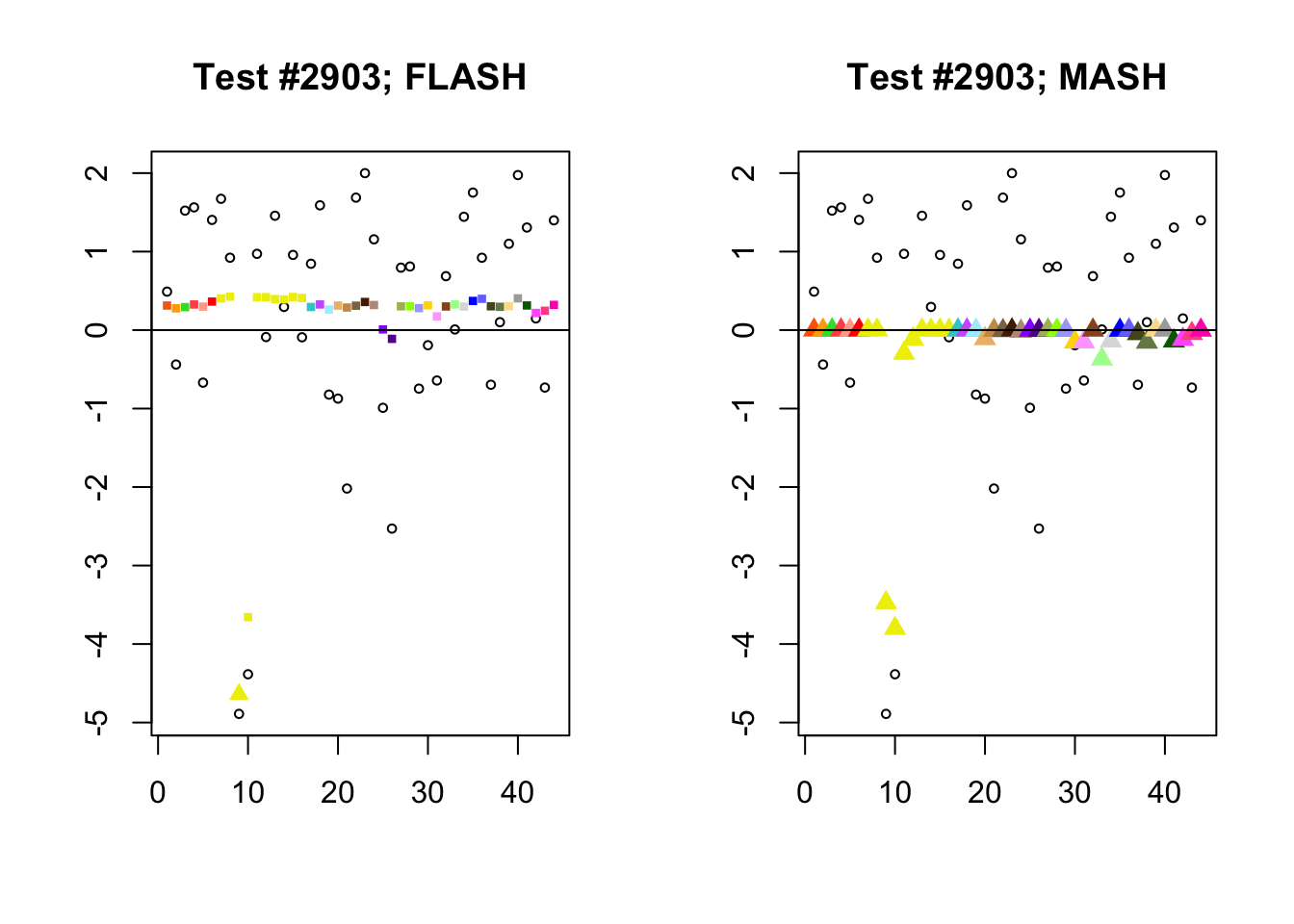
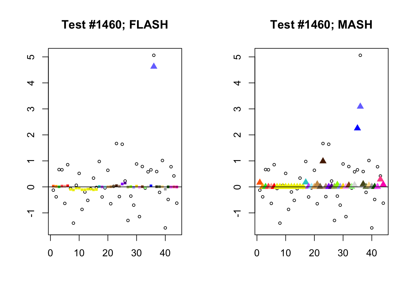
Significant for MASH, not FLASH

In many cases, MASH finds all effects to be significant where FLASH only finds a single unique effect. What happens in these cases, I think, is that MASH puts nearly all posterior weight on a single data-driven covariance matrix. Since these covariance matrices are each rank-one with no entries that are exactly equal to zero, even tiny effects will appear significant (since they are sampled away from zero nearly all of the time).

In contrast, since the FLASH model allows for covariance structures that are linear combinations of these rank-one matrices, the FLASH posteriors are far less likely to follow these patterns of perfect correlation.

par(mfrow=c(1, 2))

mash.not.flash <- c(228, 65, 2903, 1460)
for (n in mash.not.flash) {
  plot_test(n, fl_lfsr, fl_pm, "FLASH")
  plot_test(n, m_lfsr, m_pm, "MASH")
}

Expand here to see past versions of mash_not_flash-1.png:

Version	Author	Date
48615e4	Jason Willwerscheid	2018-08-15

Expand here to see past versions of mash_not_flash-2.png:

Version	Author	Date
48615e4	Jason Willwerscheid	2018-08-15

Expand here to see past versions of mash_not_flash-3.png:

Version	Author	Date
48615e4	Jason Willwerscheid	2018-08-15

Expand here to see past versions of mash_not_flash-4.png:

Version	Author	Date
48615e4	Jason Willwerscheid	2018-08-15

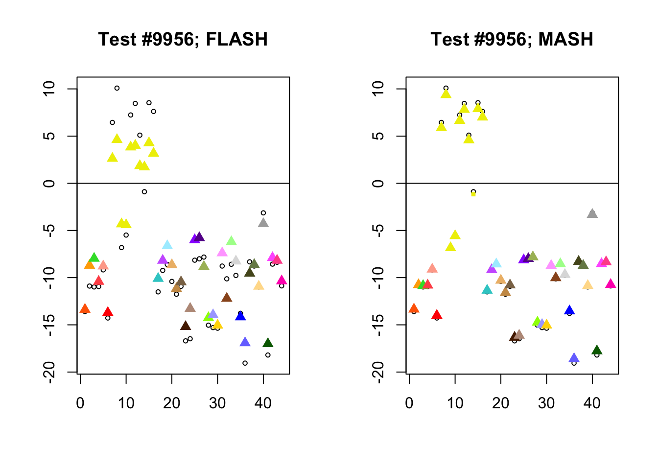
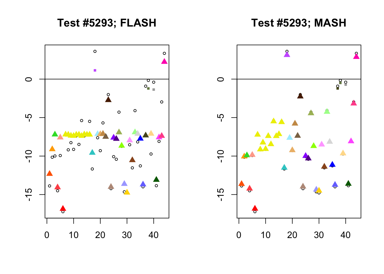
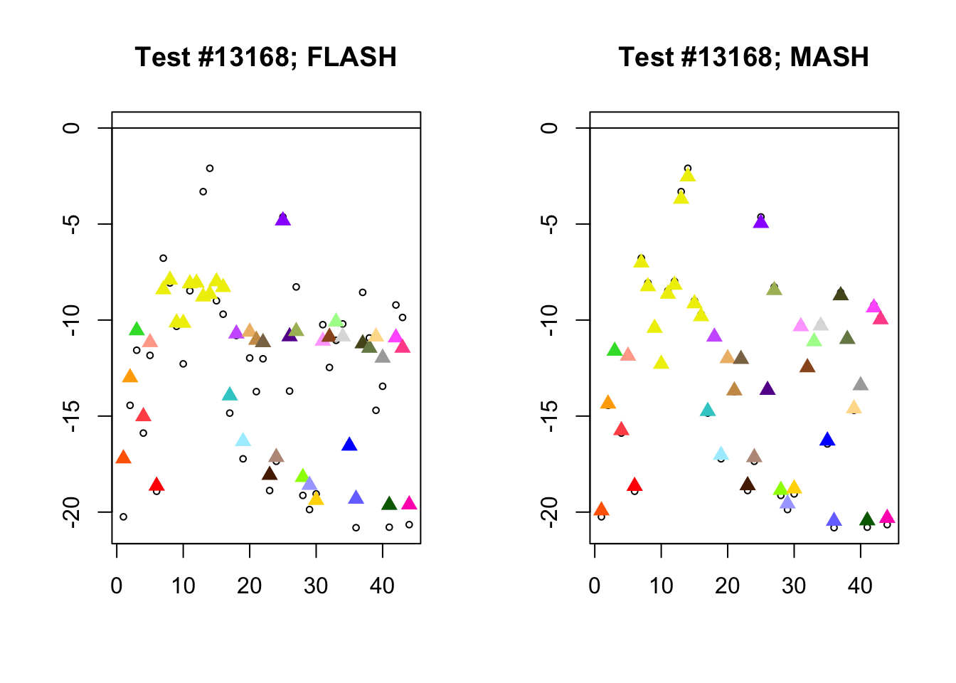
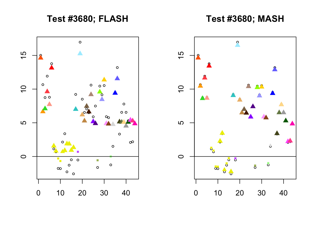
Different posterior means

As discussed here, MASH often does poorly when effect sizes are uniformly large.

par(mfrow=c(1, 2))

diff_pms <- c(9956, 5293, 13168, 3680)
for (n in diff_pms) {
  plot_test(n, fl_lfsr, fl_pm, "FLASH")
  plot_test(n, m_lfsr, m_pm, "MASH")
}

Expand here to see past versions of diff_pms-1.png:

Version	Author	Date
48615e4	Jason Willwerscheid	2018-08-15

Expand here to see past versions of diff_pms-2.png:

Version	Author	Date
48615e4	Jason Willwerscheid	2018-08-15

Expand here to see past versions of diff_pms-3.png:

Version	Author	Date
48615e4	Jason Willwerscheid	2018-08-15

Expand here to see past versions of diff_pms-4.png:

Version	Author	Date
48615e4	Jason Willwerscheid	2018-08-15

Code

Click “Code” to view the code used to obtain the fits used in this analysis.

# devtools::install_github("stephenslab/flashr")
devtools::load_all("/Users/willwerscheid/GitHub/flashr/")
# devtools::install_github("stephenslab/ebnm")
devtools::load_all("/Users/willwerscheid/GitHub/ebnm/")

library(mashr)
source("./code/utils.R")

gtex <- readRDS(gzcon(url("https://github.com/stephenslab/gtexresults/blob/master/data/MatrixEQTLSumStats.Portable.Z.rds?raw=TRUE")))

strong <- t(gtex$strong.z)
random <- t(gtex$random.z)

strong_data <- flash_set_data(strong, S = 1)
random_data <- flash_set_data(random, S = 1)

# The multi-tissue effects from the previous analysis will serve as
#   the data-driven loadings:
nn <- readRDS("./output/MASHvFLASHnn/fl.rds")
multi <- c(2, 5, 6, 8, 11:13, 17, 22:25, 31)
n <- nrow(strong)
dd <- nn$EL[, multi]
dd <- dd / rep(apply(dd, 2, max), each=n) # normalize


## FLASH fit ------------------------------------------------------------

canonical <- cbind(rep(1, n), diag(rep(1, n)))
LL <- cbind(canonical, dd)

fl_random <- flash_add_fixed_loadings(random_data, LL)
system.time(
  fl_random <- flash_backfit(random_data,
                             fl_random,
                             var_type = "zero",
                             ebnm_fn = "ebnm_pn",
                             nullcheck = FALSE)
)
# 26 minutes (62 iterations)
saveRDS(fl_random$gf, "./output/MASHvFLASHgtex3/flgf.rds")

gf <- readRDS("./output/MASHvFLASHgtex3/flgf.rds")
fl_final <- flash_add_fixed_loadings(strong_data, LL)
ebnm_param_f = lapply(gf, function(g) {list(g=g, fixg=TRUE)})
system.time(
  fl_final <- flash_backfit(strong_data,
                            fl_final,
                            var_type = "zero",
                            ebnm_fn = "ebnm_pn",
                            ebnm_param = list(f = ebnm_param_f, l = list()),
                            nullcheck = FALSE)
)
# 21 minutes (75 iterations)
saveRDS(fl_final, "./output/MASHvFLASHgtex3/fl.rds")

nsamp <- 200
system.time({
  sampler <- flash_sampler(strong_data, fl_final, fixed="loadings")
  samp <- sampler(200)
  fl_lfsr <- flash_lfsr(samp)
})
# 2 minutes
saveRDS(fl_lfsr, "./output/MASHvFLASHgtex3/fllfsr.rds")


# MASH fit --------------------------------------------------------------

strong_data <- mash_set_data(t(strong), Shat = 1)
random_data <- mash_set_data(t(random), Shat = 1)

U.flash <- list()
for (i in 1:ncol(dd)) {
  U.flash[[i]] <- outer(dd[, i], dd[, i])
}
U.c <- cov_canonical(random_data)
system.time(m_random <- mash(random_data, Ulist = c(U.c, U.flash)))
# 4 minutes

system.time(
  m_final <- mash(strong_data, g=get_fitted_g(m_random), fixg=TRUE)
)
saveRDS(m_final, "./output/MASHvFLASHgtex3/m.rds")
# 19 seconds

Session information

sessionInfo()

R version 3.4.3 (2017-11-30)
Platform: x86_64-apple-darwin15.6.0 (64-bit)
Running under: macOS High Sierra 10.13.6

Matrix products: default
BLAS: /Library/Frameworks/R.framework/Versions/3.4/Resources/lib/libRblas.0.dylib
LAPACK: /Library/Frameworks/R.framework/Versions/3.4/Resources/lib/libRlapack.dylib

locale:
[1] en_US.UTF-8/en_US.UTF-8/en_US.UTF-8/C/en_US.UTF-8/en_US.UTF-8

attached base packages:
[1] stats     graphics  grDevices utils     datasets  methods   base     

other attached packages:
[1] flashr_0.5-14 mashr_0.2-7   ashr_2.2-10  

loaded via a namespace (and not attached):
 [1] Rcpp_0.12.17        pillar_1.2.1        compiler_3.4.3     
 [4] git2r_0.21.0        plyr_1.8.4          workflowr_1.0.1    
 [7] R.methodsS3_1.7.1   R.utils_2.6.0       iterators_1.0.9    
[10] tools_3.4.3         testthat_2.0.0      digest_0.6.15      
[13] tibble_1.4.2        gtable_0.2.0        evaluate_0.10.1    
[16] memoise_1.1.0       lattice_0.20-35     rlang_0.2.0        
[19] Matrix_1.2-12       foreach_1.4.4       commonmark_1.4     
[22] yaml_2.1.17         parallel_3.4.3      ebnm_0.1-12        
[25] mvtnorm_1.0-7       xml2_1.2.0          withr_2.1.1.9000   
[28] stringr_1.3.0       knitr_1.20          roxygen2_6.0.1.9000
[31] devtools_1.13.4     rprojroot_1.3-2     grid_3.4.3         
[34] R6_2.2.2            rmarkdown_1.8       rmeta_3.0          
[37] ggplot2_2.2.1       magrittr_1.5        whisker_0.3-2      
[40] scales_0.5.0        backports_1.1.2     codetools_0.2-15   
[43] htmltools_0.3.6     MASS_7.3-48         assertthat_0.2.0   
[46] softImpute_1.4      colorspace_1.3-2    stringi_1.1.6      
[49] lazyeval_0.2.1      munsell_0.4.3       doParallel_1.0.11  
[52] pscl_1.5.2          truncnorm_1.0-8     SQUAREM_2017.10-1  
[55] R.oo_1.21.0