Nonnegative loadings with non-diagonal V
Last updated: 2018-09-05
workflowr checks: (Click a bullet for more information)-
✔ R Markdown file: up-to-date
Great! Since the R Markdown file has been committed to the Git repository, you know the exact version of the code that produced these results.
-
✔ Environment: empty
Great job! The global environment was empty. Objects defined in the global environment can affect the analysis in your R Markdown file in unknown ways. For reproduciblity it’s best to always run the code in an empty environment.
-
✔ Seed:
set.seed(20180609)The command
set.seed(20180609)was run prior to running the code in the R Markdown file. Setting a seed ensures that any results that rely on randomness, e.g. subsampling or permutations, are reproducible. -
✔ Session information: recorded
Great job! Recording the operating system, R version, and package versions is critical for reproducibility.
-
Great! You are using Git for version control. Tracking code development and connecting the code version to the results is critical for reproducibility. The version displayed above was the version of the Git repository at the time these results were generated.✔ Repository version: d17ac04
Note that you need to be careful to ensure that all relevant files for the analysis have been committed to Git prior to generating the results (you can usewflow_publishorwflow_git_commit). workflowr only checks the R Markdown file, but you know if there are other scripts or data files that it depends on. Below is the status of the Git repository when the results were generated:
Note that any generated files, e.g. HTML, png, CSS, etc., are not included in this status report because it is ok for generated content to have uncommitted changes.Ignored files: Ignored: .DS_Store Ignored: .Rhistory Ignored: .Rproj.user/ Ignored: data/ Ignored: docs/.DS_Store Ignored: docs/images/.DS_Store Ignored: docs/images/.Rapp.history Ignored: output/.DS_Store Ignored: output/.Rapp.history Ignored: output/MASHvFLASHgtex/.DS_Store Ignored: output/MASHvFLASHsims/.DS_Store Ignored: output/MASHvFLASHsims/backfit/.DS_Store Ignored: output/MASHvFLASHsims/backfit/.Rapp.history Untracked files: Untracked: code/MASHvFLASHnn2.R Untracked: code/MASHvFLASHnnrefine.R Untracked: output/MASHvFLASHnn2/
Expand here to see past versions:
| File | Version | Author | Date | Message |
|---|---|---|---|---|
| Rmd | d17ac04 | Jason Willwerscheid | 2018-09-05 | wflow_publish(“analysis/MASHvFLASHnondiagonalV.Rmd”) |
| html | 603daf1 | Jason Willwerscheid | 2018-08-30 | Build site. |
| Rmd | 4ca600b | Jason Willwerscheid | 2018-08-30 | wflow_publish(c(“analysis/MASHvFLASHnondiagonalV.Rmd”, |
| html | fb53e92 | Jason Willwerscheid | 2018-08-30 | Build site. |
| Rmd | 861ba07 | Jason Willwerscheid | 2018-08-30 | wflow_publish(“analysis/MASHvFLASHnondiagonalV.Rmd”) |
| html | 273efe5 | Jason Willwerscheid | 2018-08-30 | Build site. |
| Rmd | fad7859 | Jason Willwerscheid | 2018-08-30 | wflow_publish(“analysis/MASHvFLASHnondiagonalV.Rmd”) |
Introduction
Here I again fit nonnegative loadings to the “strong” GTEx dataset, but I now use the trick discussed here to fit a non-diagonal error covariance matrix \(V\).
I pre-run the code below and load the results from file.
Comparison with previous results
Whereas my earlier analysis (which implicitly assumed that \(V = I\)) found 39 data-driven loadings, here I was only able to obtain 26.
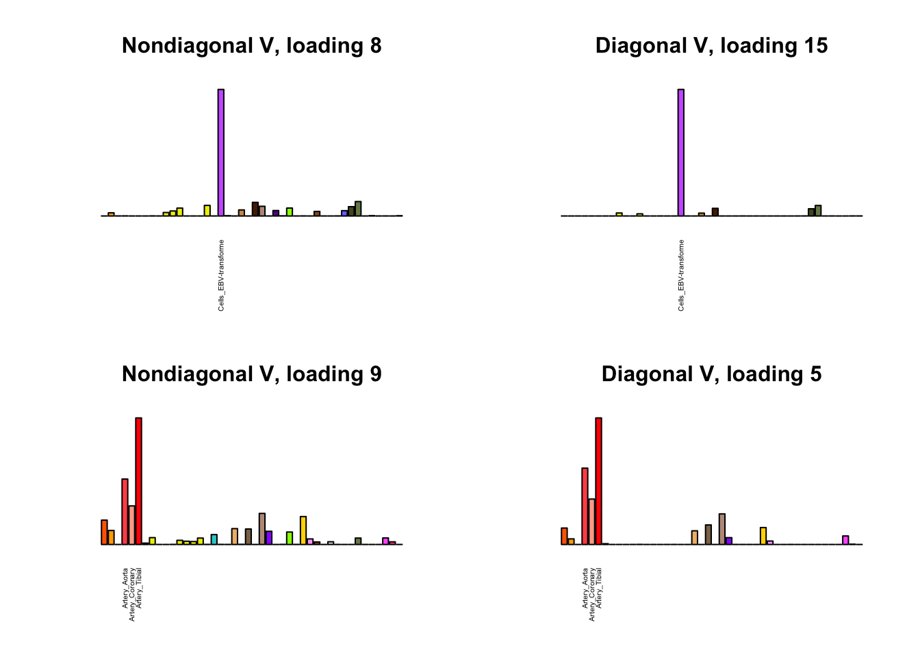
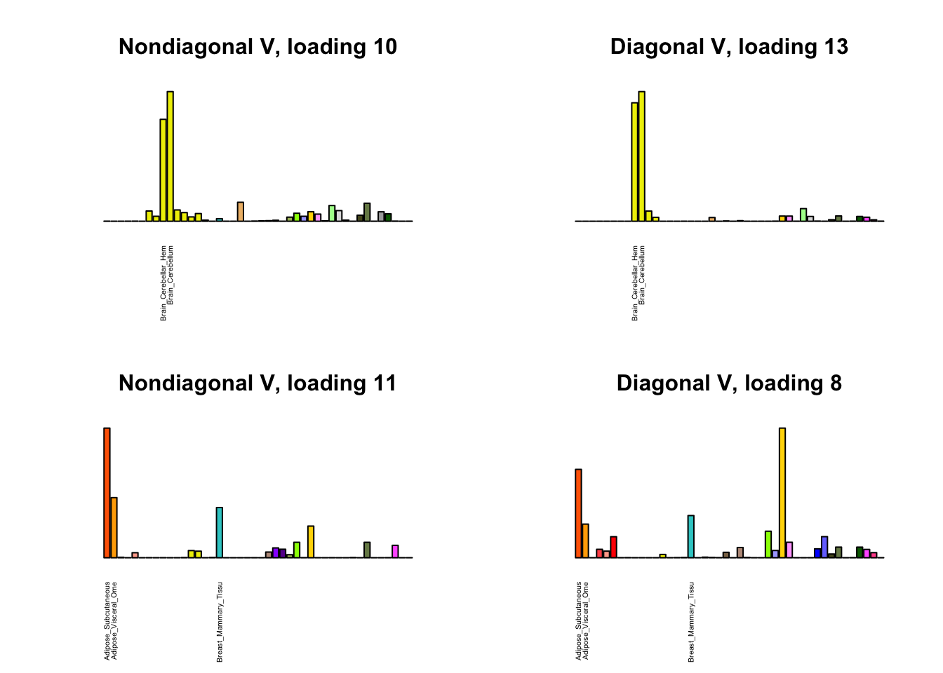
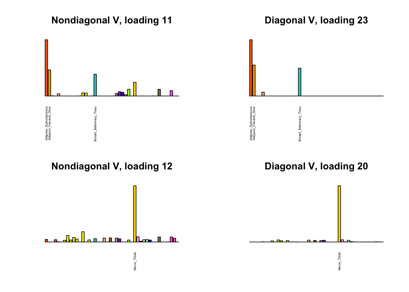
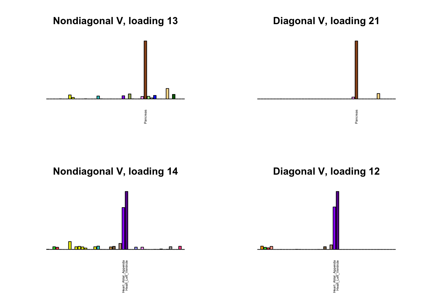
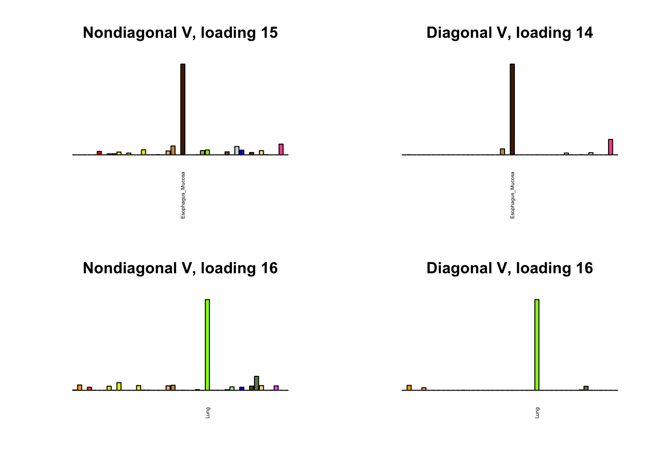
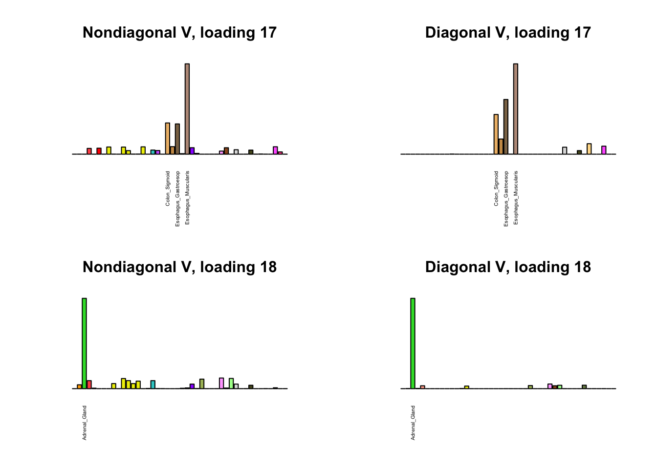
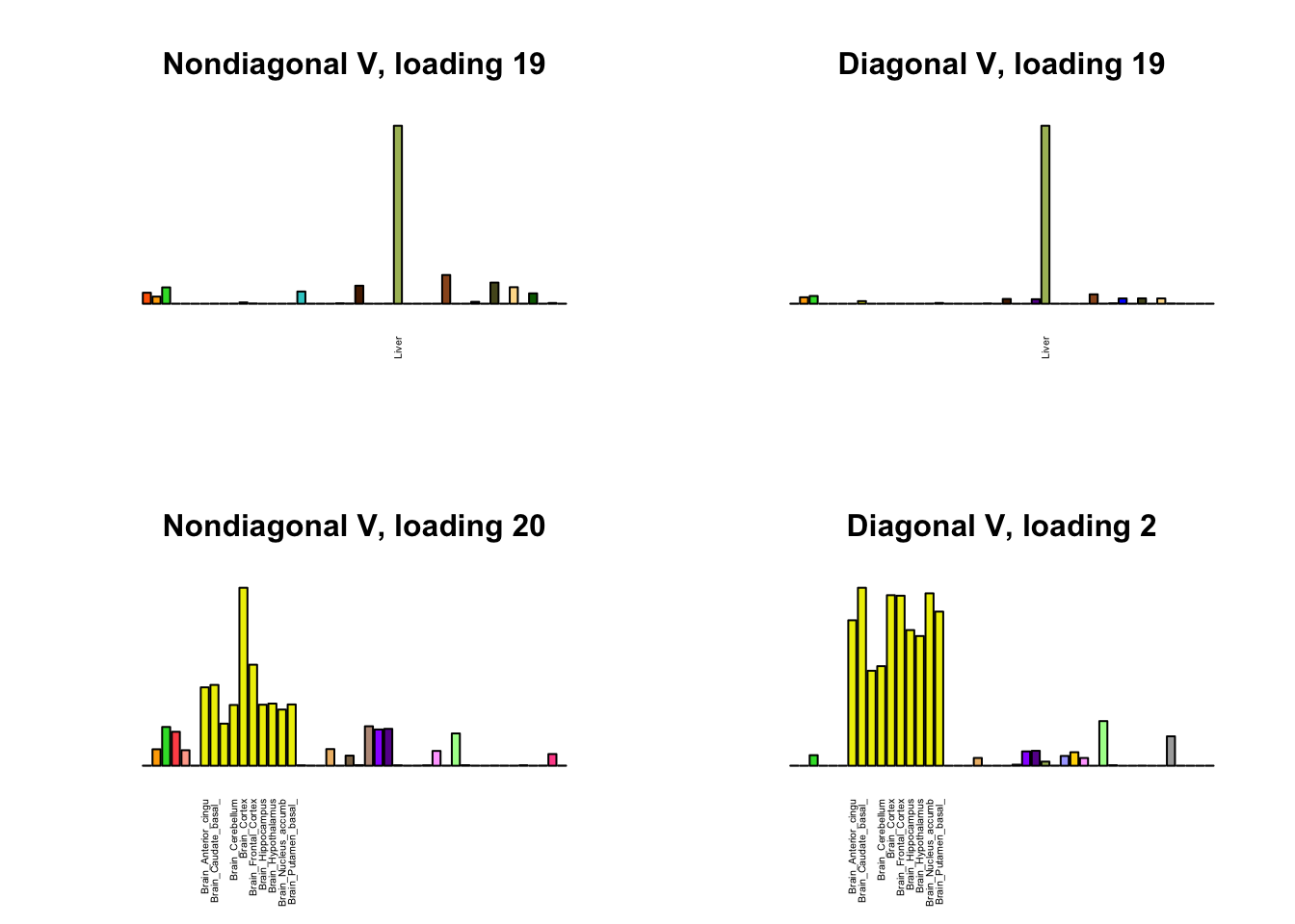
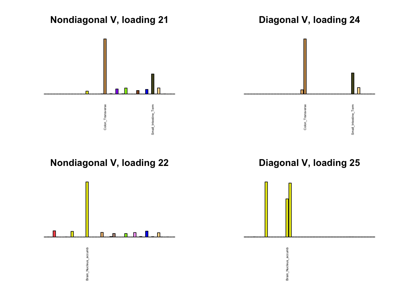
Similar loadings
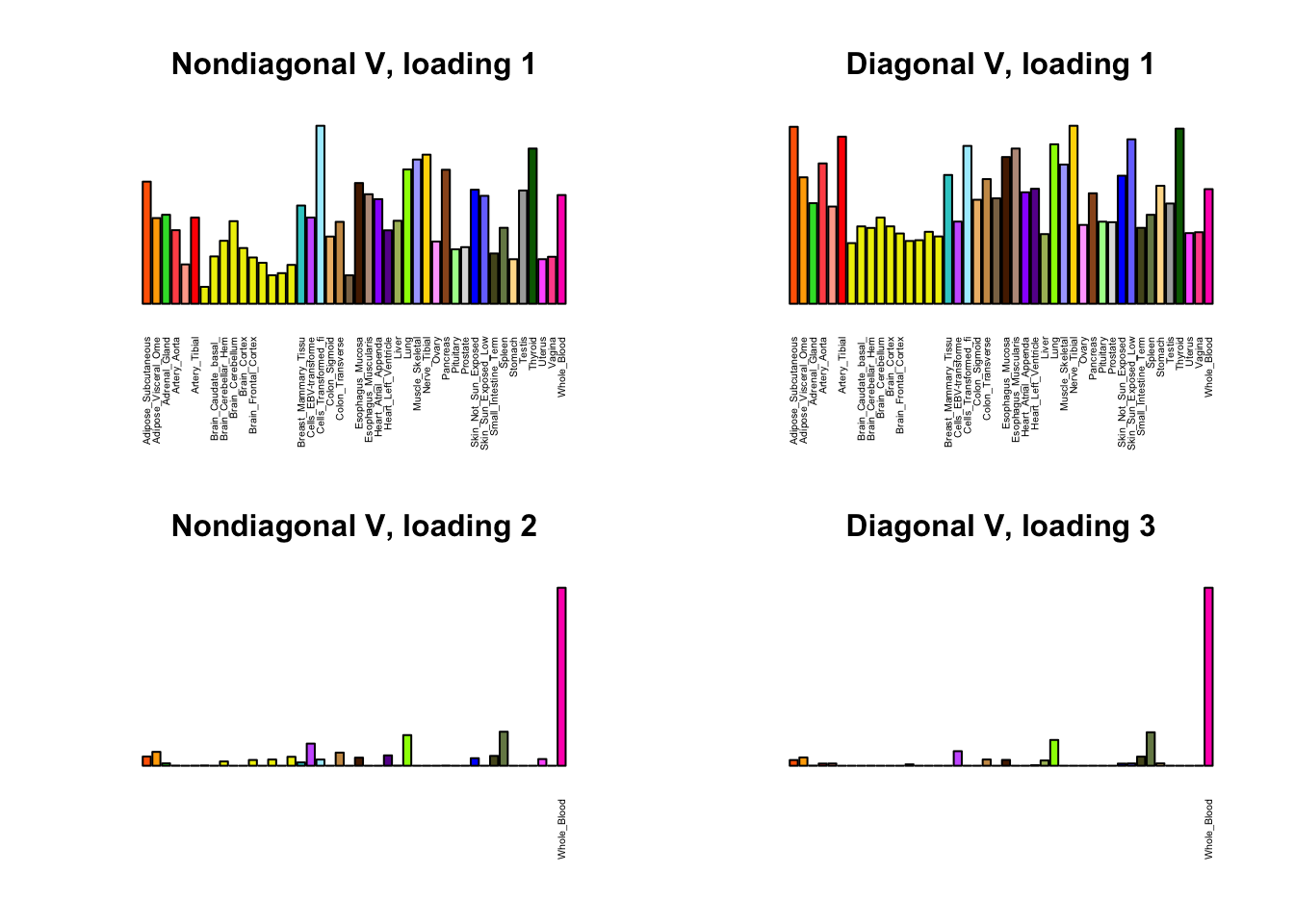
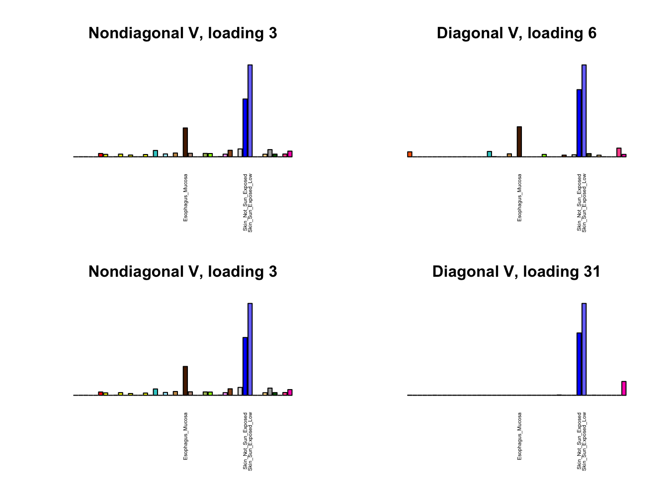
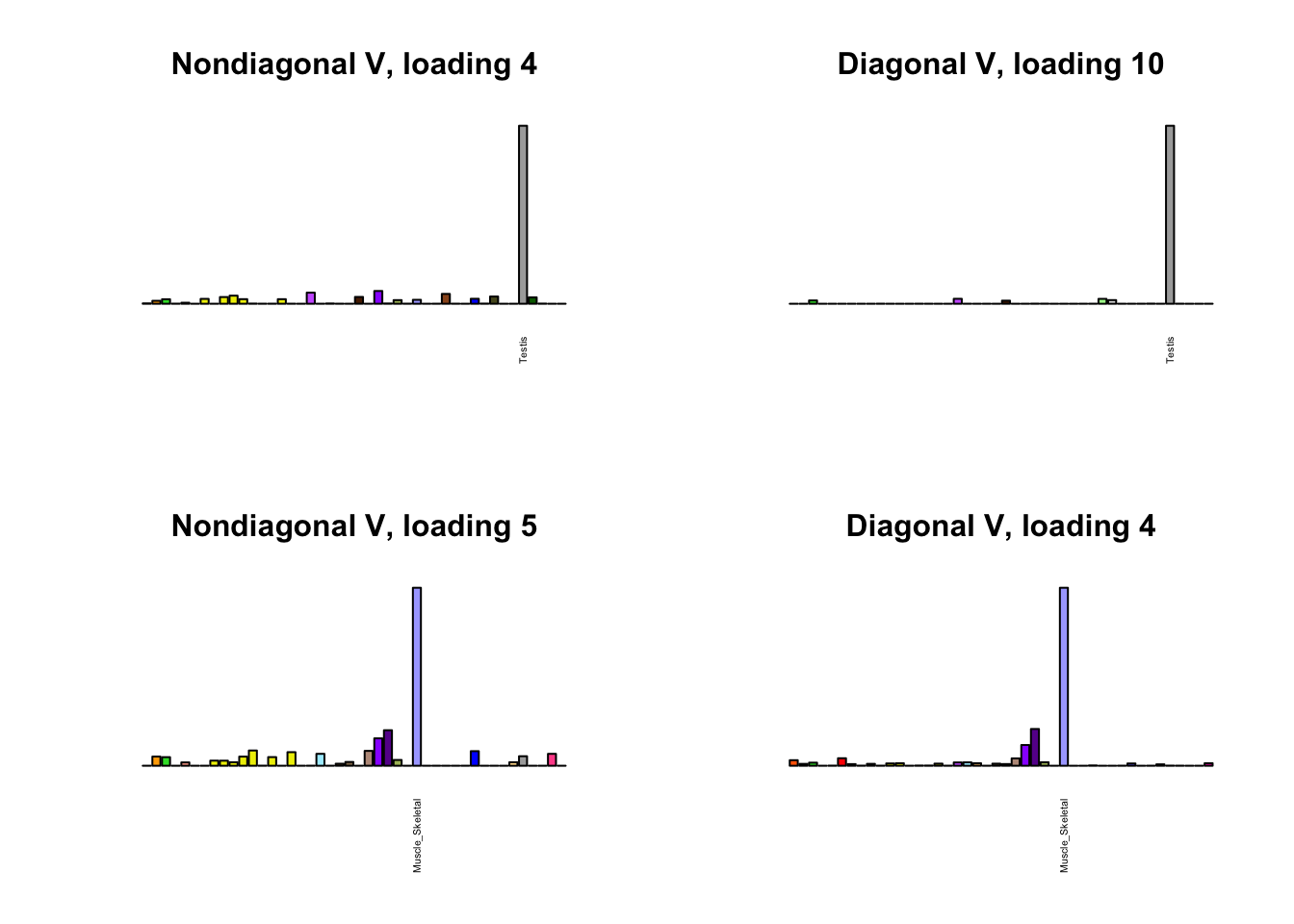
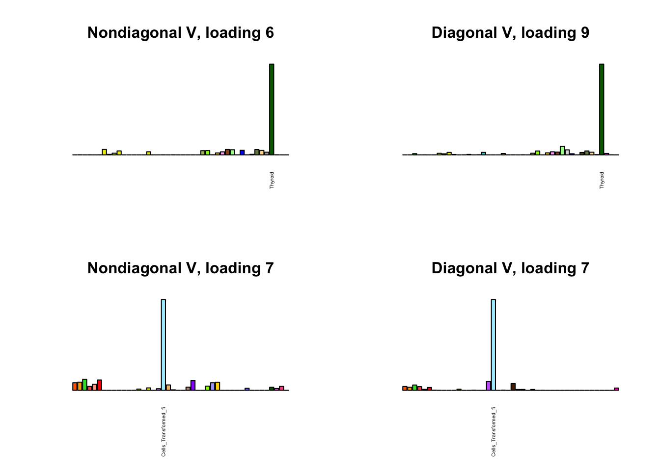
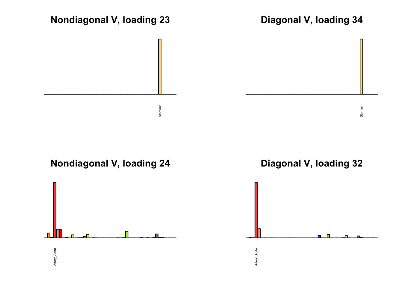
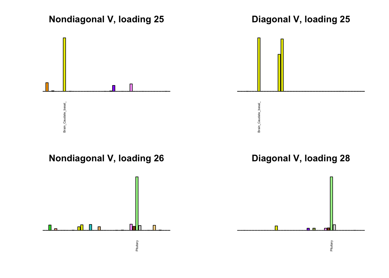
I first plot the new loadings side by side with the previous loadings to which they most closely correspond. Note that, in general, the previous loadings tend to be sparser than these new loadings. Further, this new approach finds two unique effects (caudate basal ganglia and nucleus accumbens basal ganglia) where the previous approach very plausibly found correlations among three types of basal ganglia (loading 25). However, the adipose tissue effects (loading 11) do not get tangled up with the tibial nerve tissue effect (as they did in the previous approach), and there is a single loading describing correlations among skin tissues (loading 3) rather than two largely overlapping loadings.
nondiag <- readRDS("./output/MASHvFLASHnondiagonalV/2dRepeat3.rds")
diag <- readRDS("./output/MASHvFLASHnn/fl.rds")

nondiag_order <- c(44:46, 46:54, 54:nondiag$nfactors)
diag_order <- c(1, 3, 6, 31, 10,
                4, 9, 7, 15,
                5, 13, 8, 23, 20,
                21, 12, 14, 16,
                17, 18, 19, 2,
                24, 25, 34, 32,
                25, 28)

diag_not_nondiag <- setdiff(c(1:29, 32:40), diag_order)

tissue_names <- rownames(diag$EL)

missing.tissues <- c(7, 8, 19, 20, 24, 25, 31, 34, 37)
gtex.colors <- read.table("https://github.com/stephenslab/gtexresults/blob/master/data/GTExColors.txt?raw=TRUE", sep = '\t', comment.char = '')[-missing.tissues, 2]
gtex.colors <- as.character(gtex.colors)

par(mfrow=c(2,2))
display_names <- strtrim(tissue_names, 20)
for(i in 1:length(nondiag_order)) {
  plot_names <- display_names

  next_nondiag <- nondiag$fit$EL[, nondiag_order[i]]
  plot_names[next_nondiag < 0.25 * max(next_nondiag)] <- ""
  barplot(next_nondiag,
          main=paste0('Nondiagonal V, loading ', nondiag_order[i] - 43),
          las=2, cex.names=0.4, yaxt='n',
          col=gtex.colors, names=plot_names)

  barplot(diag$EL[, diag_order[i]],
          main=paste0('Diagonal V, loading ', diag_order[i]),
          las=2, cex.names=0.4, yaxt='n',
          col=gtex.colors, names=plot_names)
}
Expand here to see past versions of shared-1.png:
| Version | Author | Date |
|---|---|---|
| 273efe5 | Jason Willwerscheid | 2018-08-30 |
Expand here to see past versions of shared-2.png:
| Version | Author | Date |
|---|---|---|
| 273efe5 | Jason Willwerscheid | 2018-08-30 |
Expand here to see past versions of shared-3.png:
| Version | Author | Date |
|---|---|---|
| 273efe5 | Jason Willwerscheid | 2018-08-30 |
Expand here to see past versions of shared-4.png:
| Version | Author | Date |
|---|---|---|
| 273efe5 | Jason Willwerscheid | 2018-08-30 |
Expand here to see past versions of shared-5.png:
| Version | Author | Date |
|---|---|---|
| 273efe5 | Jason Willwerscheid | 2018-08-30 |
Expand here to see past versions of shared-6.png:
| Version | Author | Date |
|---|---|---|
| 273efe5 | Jason Willwerscheid | 2018-08-30 |
Expand here to see past versions of shared-7.png:
| Version | Author | Date |
|---|---|---|
| 273efe5 | Jason Willwerscheid | 2018-08-30 |
Expand here to see past versions of shared-8.png:
| Version | Author | Date |
|---|---|---|
| 273efe5 | Jason Willwerscheid | 2018-08-30 |
Expand here to see past versions of shared-9.png:
| Version | Author | Date |
|---|---|---|
| 273efe5 | Jason Willwerscheid | 2018-08-30 |
Expand here to see past versions of shared-10.png:
| Version | Author | Date |
|---|---|---|
| 273efe5 | Jason Willwerscheid | 2018-08-30 |
Expand here to see past versions of shared-11.png:
| Version | Author | Date |
|---|---|---|
| 273efe5 | Jason Willwerscheid | 2018-08-30 |
Expand here to see past versions of shared-12.png:
| Version | Author | Date |
|---|---|---|
| 273efe5 | Jason Willwerscheid | 2018-08-30 |
Expand here to see past versions of shared-13.png:
| Version | Author | Date |
|---|---|---|
| 273efe5 | Jason Willwerscheid | 2018-08-30 |
Expand here to see past versions of shared-14.png:
| Version | Author | Date |
|---|---|---|
| 273efe5 | Jason Willwerscheid | 2018-08-30 |
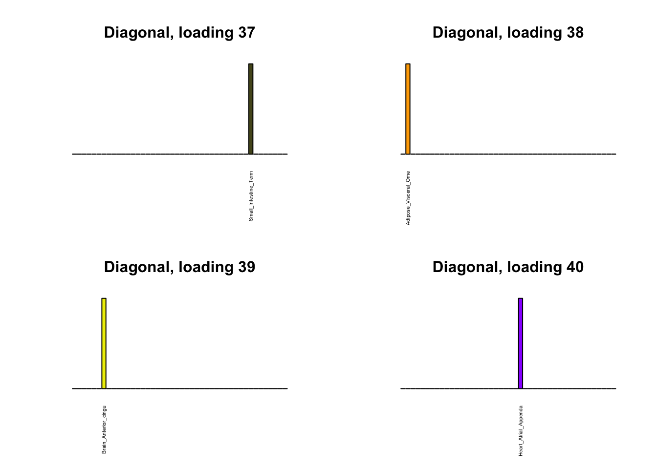
Differences
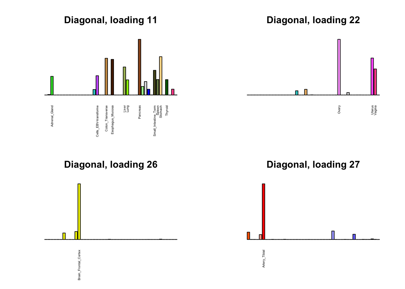
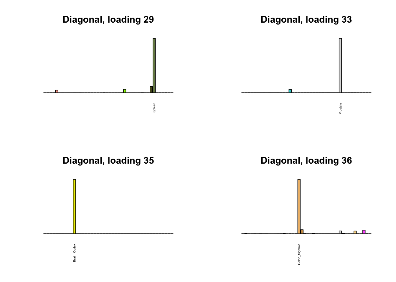
Next, I plot previous loadings that do not correspond to any of the new loadings. One of these (loading 11) may indeed be an artefactual loading that corresponds to covariance in errors rather than biological reality. However, one of the others (loading 22) describes a plausible correlation among ovarian, uterine, and vaginal tissues. The remaining are unique effects.
par(mfrow=c(2,2))
for (i in 1:length(diag_not_nondiag)) {
  plot_names <- display_names

  next_diag <- diag$EL[, diag_not_nondiag[i]]
  plot_names[next_diag < 0.25 * max(next_diag)] <- ""
  barplot(next_diag,
          main=paste0('Diagonal, loading ', diag_not_nondiag[i]),
          las=2, cex.names=0.4, yaxt='n',
          col=gtex.colors, names=plot_names)
}
Expand here to see past versions of extra-1.png:
| Version | Author | Date |
|---|---|---|
| 273efe5 | Jason Willwerscheid | 2018-08-30 |
Expand here to see past versions of extra-2.png:
| Version | Author | Date |
|---|---|---|
| 273efe5 | Jason Willwerscheid | 2018-08-30 |
Expand here to see past versions of extra-3.png:
| Version | Author | Date |
|---|---|---|
| 273efe5 | Jason Willwerscheid | 2018-08-30 |
Code
Click “Code” to view the code used to obtain the above results.
devtools::load_all("/Users/willwerscheid/GitHub/flashr/")
devtools::load_all("/Users/willwerscheid/GitHub/ebnm/")

library(mashr)

gtex <- readRDS(gzcon(url("https://github.com/stephenslab/gtexresults/blob/master/data/MatrixEQTLSumStats.Portable.Z.rds?raw=TRUE")))

strong <- gtex$strong.z
random <- gtex$random.z

# Step 1. Estimate correlation structure using MASH.

m_random <- mash_set_data(random, Shat = 1)
Vhat <- estimate_null_correlation(m_random)

# Step 2. Estimate data-driven loadings using FLASH.

# Step 2a. Fit Vhat.
n <- nrow(Vhat)
lambda.min <- min(eigen(Vhat, symmetric=TRUE, only.values=TRUE)$values)

data <- flash_set_data(Y, S = sqrt(lambda.min))

W.eigen <- eigen(Vhat - diag(rep(lambda.min, n)), symmetric=TRUE)
# The rank of W is at most n - 1, so we can drop the last eigenval/vec:
W.eigen$values <- W.eigen$values[-n]
W.eigen$vectors <- W.eigen$vectors[, -n, drop=FALSE]

fl <- flash_add_fixed_loadings(data,
                               LL=W.eigen$vectors,
                               init_fn="udv_svd",
                               backfit=FALSE)

ebnm_param_f <- lapply(as.list(W.eigen$values),
                       function(eigenval) {
                         list(g = list(a=1/eigenval, pi0=0), fixg = TRUE)
                       })
ebnm_param_l <- lapply(vector("list", n - 1),
                       function(k) {list()})
fl <- flash_backfit(data,
                    fl,
                    var_type="zero",
                    ebnm_fn="ebnm_pn",
                    ebnm_param=(list(f = ebnm_param_f, l = ebnm_param_l)),
                    nullcheck=FALSE)

# Step 2b. Add nonnegative factors.
ebnm_fn = list(f = "ebnm_pn", l = "ebnm_ash")
ebnm_param = list(f = list(warmstart = TRUE),
                  l = list(mixcompdist="+uniform"))
fl <- flash_add_greedy(data,
                       Kmax=50,
                       f_init=fl,
                       var_type="zero",
                       init_fn="udv_svd",
                       ebnm_fn=ebnm_fn,
                       ebnm_param=ebnm_param)
saveRDS(fl, "./output/MASHvFLASHVhat/2bGreedy.rds")

# Step 2c (optional). Backfit factors from step 2b.
fl <- flash_backfit(data,
                    fl,
                    kset=n:fl$nfactors,
                    var_type="zero",
                    ebnm_fn=ebnm_fn,
                    ebnm_param=ebnm_param,
                    nullcheck=FALSE)
saveRDS(fl, "./output/MASHvFLASHVhat/2cBackfit.rds")

# Step 2d (optional). Repeat steps 2b and 2c as desired.
fl <- flash_add_greedy(data,
                       Kmax=50,
                       f_init=fl,
                       var_type="zero",
                       init_fn="udv_svd",
                       ebnm_fn=ebnm_fn,
                       ebnm_param=ebnm_param)
fl <- flash_backfit(data,
                    fl,
                    kset=n:fl$nfactors,
                    var_type="zero",
                    ebnm_fn=ebnm_fn,
                    ebnm_param=ebnm_param,
                    nullcheck=FALSE)
saveRDS(fl, "./output/MASHvFLASHVhat/2dRepeat3.rds")
Session information
sessionInfo()R version 3.4.3 (2017-11-30)
Platform: x86_64-apple-darwin15.6.0 (64-bit)
Running under: macOS High Sierra 10.13.6
Matrix products: default
BLAS: /Library/Frameworks/R.framework/Versions/3.4/Resources/lib/libRblas.0.dylib
LAPACK: /Library/Frameworks/R.framework/Versions/3.4/Resources/lib/libRlapack.dylib
locale:
[1] en_US.UTF-8/en_US.UTF-8/en_US.UTF-8/C/en_US.UTF-8/en_US.UTF-8
attached base packages:
[1] stats graphics grDevices utils datasets methods base
loaded via a namespace (and not attached):
[1] workflowr_1.0.1 Rcpp_0.12.17 digest_0.6.15
[4] rprojroot_1.3-2 R.methodsS3_1.7.1 backports_1.1.2
[7] git2r_0.21.0 magrittr_1.5 evaluate_0.10.1
[10] stringi_1.1.6 whisker_0.3-2 R.oo_1.21.0
[13] R.utils_2.6.0 rmarkdown_1.8 tools_3.4.3
[16] stringr_1.3.0 yaml_2.1.17 compiler_3.4.3
[19] htmltools_0.3.6 knitr_1.20 This reproducible R Markdown analysis was created with workflowr 1.0.1