Nonnegative FLASH loadings (redux)
Last updated: 2018-09-21
workflowr checks: (Click a bullet for more information)-
✔ R Markdown file: up-to-date
Great! Since the R Markdown file has been committed to the Git repository, you know the exact version of the code that produced these results.
-
✔ Environment: empty
Great job! The global environment was empty. Objects defined in the global environment can affect the analysis in your R Markdown file in unknown ways. For reproduciblity it’s best to always run the code in an empty environment.
-
✔ Seed:
set.seed(20180609)The command
set.seed(20180609)was run prior to running the code in the R Markdown file. Setting a seed ensures that any results that rely on randomness, e.g. subsampling or permutations, are reproducible. -
✔ Session information: recorded
Great job! Recording the operating system, R version, and package versions is critical for reproducibility.
-
Great! You are using Git for version control. Tracking code development and connecting the code version to the results is critical for reproducibility. The version displayed above was the version of the Git repository at the time these results were generated.✔ Repository version: ade96ef
Note that you need to be careful to ensure that all relevant files for the analysis have been committed to Git prior to generating the results (you can usewflow_publishorwflow_git_commit). workflowr only checks the R Markdown file, but you know if there are other scripts or data files that it depends on. Below is the status of the Git repository when the results were generated:
Note that any generated files, e.g. HTML, png, CSS, etc., are not included in this status report because it is ok for generated content to have uncommitted changes.Ignored files: Ignored: .DS_Store Ignored: .Rhistory Ignored: .Rproj.user/ Ignored: data/ Ignored: docs/.DS_Store Ignored: docs/images/.DS_Store Ignored: docs/images/.Rapp.history Ignored: output/.DS_Store Ignored: output/.Rapp.history Ignored: output/MASHvFLASHgtex/.DS_Store Ignored: output/MASHvFLASHsims/.DS_Store Ignored: output/MASHvFLASHsims/backfit/.DS_Store Ignored: output/MASHvFLASHsims/backfit/.Rapp.history Untracked files: Untracked: code/MASHvFLASHcorshrink.R Untracked: code/MASHvFLASHnn2.R Untracked: code/MASHvFLASHnnrefine.R Untracked: code/MASHvFLASHortho.R Untracked: output/MASHvFLASHnn2/
Expand here to see past versions:
| File | Version | Author | Date | Message |
|---|---|---|---|---|
| Rmd | ade96ef | Jason Willwerscheid | 2018-09-21 | wflow_publish(“analysis/MASHvFLASHnn2.Rmd”) |
Introduction
In a previous analysis, I used nonnegative priors to obtain a set of sparse and interpretable loadings from GTEx data. Here I repeat the analysis using the updated FLASH interface (current as of 9/21/18).
Fits
I’m not sure whether var_type = "zero" or var_type = "constant" is more appropriate, so I use both. I produce three fits for each variance type. Each builds on the previous, so that the objective is guaranteed to decrease from fit to fit:
- A single round of greedily adding factors.
- A single round of greedily adding factors, followed by backfitting (including a nullcheck).
- Repeatedly greedily adding factors and then backfitting until the greedy step no longer adds any new factors.
Results
I pre-run the code and load the results from file.
fl_g_zero <- readRDS("./output/MASHvFLASHnn2/fl_g_zero.rds")
t_g_zero <- readRDS("./output/MASHvFLASHnn2/t_g_zero.rds")
fl_b_zero <- readRDS("./output/MASHvFLASHnn2/fl_b_zero.rds")
t_b_zero <- readRDS("./output/MASHvFLASHnn2/t_b_zero.rds")
fl_g2_zero <- readRDS("./output/MASHvFLASHnn2/fl_g2_zero.rds")
t_g2_zero <- readRDS("./output/MASHvFLASHnn2/t_g2_zero.rds")
fl_b2_zero <- readRDS("./output/MASHvFLASHnn2/fl_b2_zero.rds")
t_b2_zero <- readRDS("./output/MASHvFLASHnn2/t_b2_zero.rds")
fl_g_const <- readRDS("./output/MASHvFLASHnn2/fl_g_const.rds")
t_g_const <- readRDS("./output/MASHvFLASHnn2/t_g_const.rds")
fl_b_const <- readRDS("./output/MASHvFLASHnn2/fl_b_const.rds")
t_b_const <- readRDS("./output/MASHvFLASHnn2/t_b_const.rds")
fl_g2_const <- readRDS("./output/MASHvFLASHnn2/fl_g2_const.rds")
t_g2_const <- readRDS("./output/MASHvFLASHnn2/t_g2_const.rds")
fl_b2_const <- readRDS("./output/MASHvFLASHnn2/fl_b2_const.rds")
t_b2_const <- readRDS("./output/MASHvFLASHnn2/t_b2_const.rds")
Number of factors
The number of factors included in each fit is:
nfactors <- c(fl_g_zero$nfactors,
              fl_b_zero$nfactors,
              fl_b2_zero$nfactors,
              fl_g_const$nfactors,
              fl_b_const$nfactors,
              fl_b2_const$nfactors)

arrange_res <- function(res) {
  res <- matrix(res, nrow = 3, ncol = 2)
  rownames(res) <- c("greedy", "backfit", "repeated")
  colnames(res) <- c("zero", "constant")
  return(res)
}

arrange_res(nfactors)
zero constant
greedy 34 25
backfit 33 25
repeated 40 27Runtime
The number of minutes required to fit each model (on my MacBook Pro) is:
runtime <- c(t_g_zero[3],
             t_g_zero[3] + t_b_zero[3],
             t_g_zero[3] + t_b_zero[3] + t_g2_zero[3] + t_b2_zero[3],
             t_g_const[3],
             t_g_const[3] + t_b_const[3],
             t_g_const[3] + t_b_const[3] + t_g2_const[3] + t_b2_const[3])
runtime <- round(runtime / 60, digits = 1)

arrange_res(runtime)
zero constant
greedy 5.4 3.3
backfit 20.4 16.4
repeated 41.9 26.3Objective
The objective attained by each fit, relative to the maximum objective attained among all fits, is:
obj <- c(fl_g_zero$objective,
         fl_b_zero$objective,
         fl_b2_zero$objective,
         fl_g_const$objective,
         fl_b_const$objective,
         fl_b2_const$objective)
obj <- round(obj - max(obj), digits = 0)

arrange_res(obj)
zero constant
greedy -35099 -30373
backfit -1754 -2577
repeated 0 -1139Interestingly, the “zero” variance type (where standard errors are fixed) does better than the “constant” variance type (where standard errors are estimated), simply because it is able to add more factors!
Factors
To compare qualitative results, I plot the factors from each fit side by side. I ignore factors that correspond to “unique effects.” From left to right, the factors are those produced by a greedy fit, a greedy fit with backfitting, and multiple rounds of greedy addition and backfitting.
missing.tissues <- c(7, 8, 19, 20, 24, 25, 31, 34, 37)
gtex.colors <- read.table("https://github.com/stephenslab/gtexresults/blob/master/data/GTExColors.txt?raw=TRUE", sep = '\t', comment.char = '')[-missing.tissues, 2]
gtex.colors <- as.character(gtex.colors)

zero_factors <- c(1:5, 8:12, 16:19, 21:22, 25)
const_factors <- c(1:5, 8:12, 21, 13, 16, 14, 22, 20, 24)

par(mfrow = c(2, 3))
for (k in 1:length(zero_factors)) {
  barplot(fl_g_zero$ldf$f[, zero_factors[k]], col=gtex.colors,
          names.arg = FALSE, axes = FALSE)
  barplot(fl_b_zero$ldf$f[, zero_factors[k]], col=gtex.colors,
          names.arg = FALSE, axes = FALSE,
          main = paste("Factor", zero_factors[k], "(Zero)"))
  barplot(fl_b2_zero$ldf$f[, zero_factors[k]], col=gtex.colors,
          names.arg = FALSE, axes = FALSE)
  barplot(fl_g_const$ldf$f[, const_factors[k]], col=gtex.colors,
          names.arg = FALSE, axes = FALSE)
  barplot(fl_b_const$ldf$f[, const_factors[k]], col=gtex.colors,
          names.arg = FALSE, axes = FALSE,
          main = paste("Factor", const_factors[k], "(Constant)"))
  barplot(fl_b2_const$ldf$f[, const_factors[k]], col=gtex.colors,
          names.arg = FALSE, axes = FALSE)
}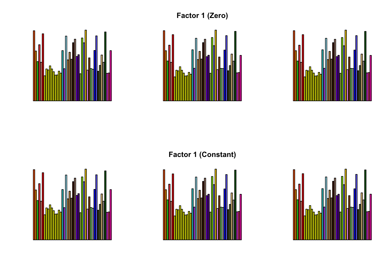
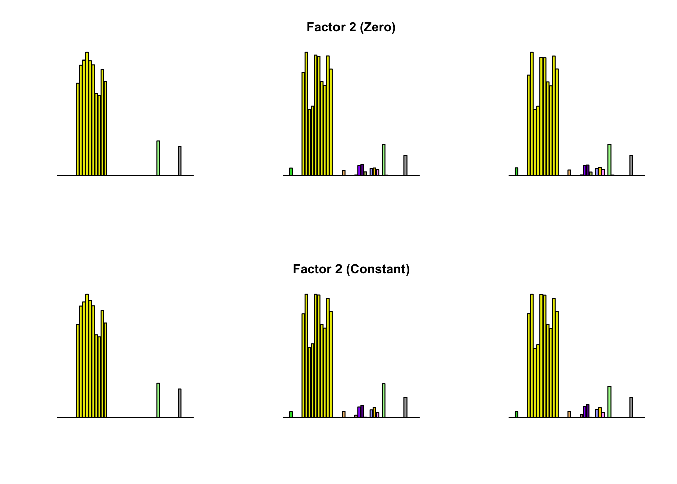
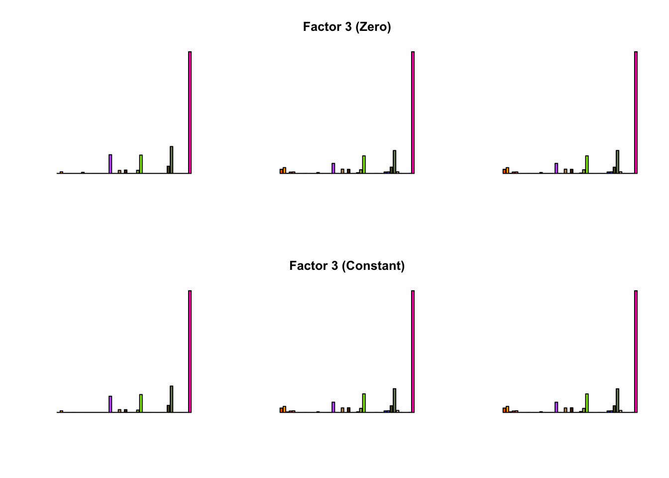
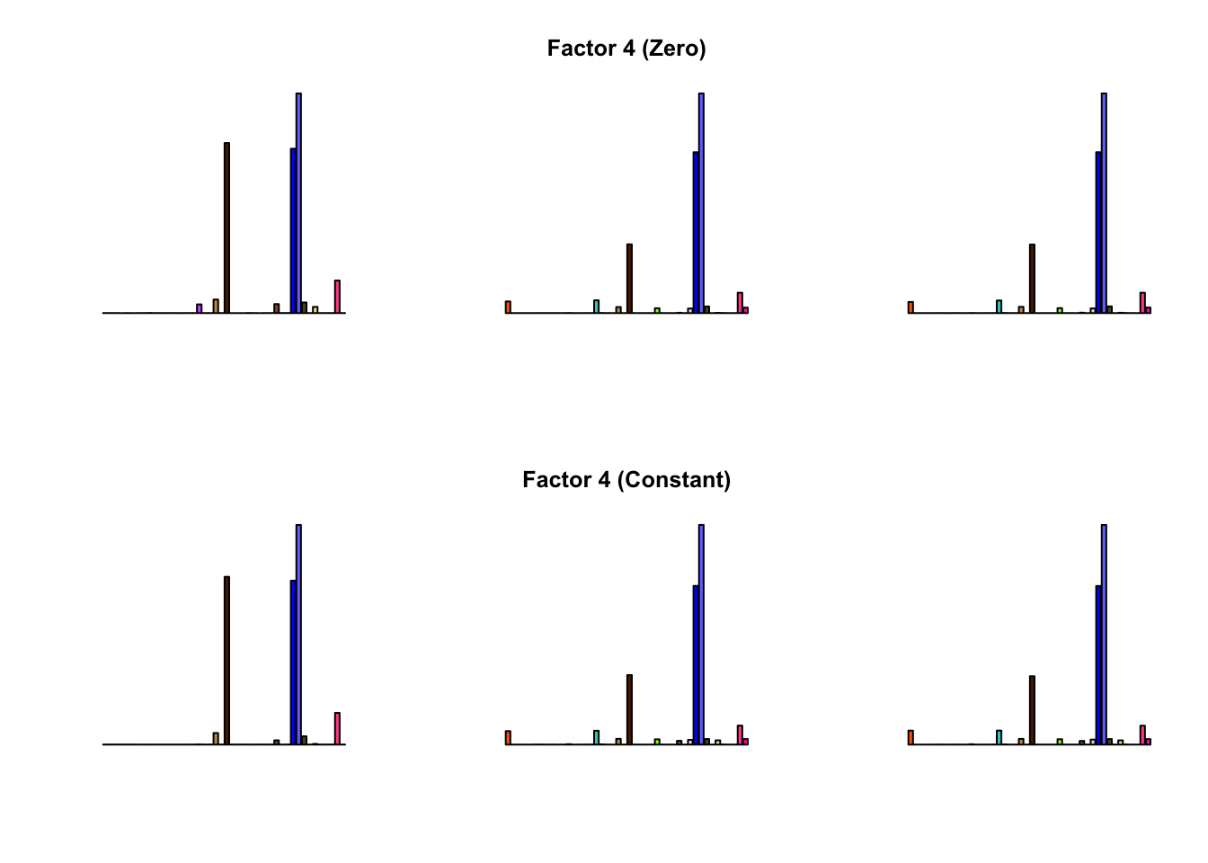
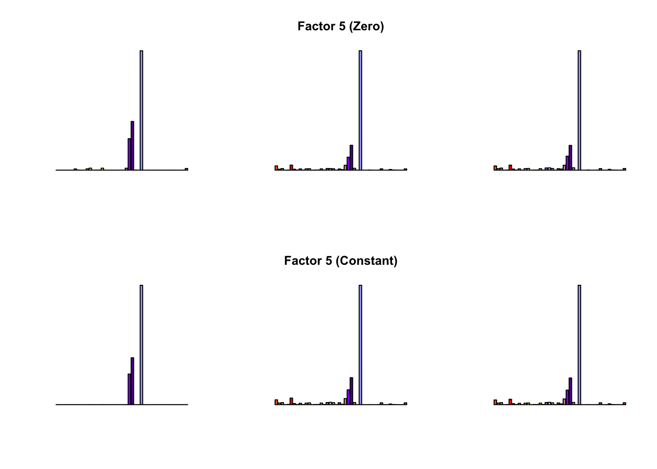
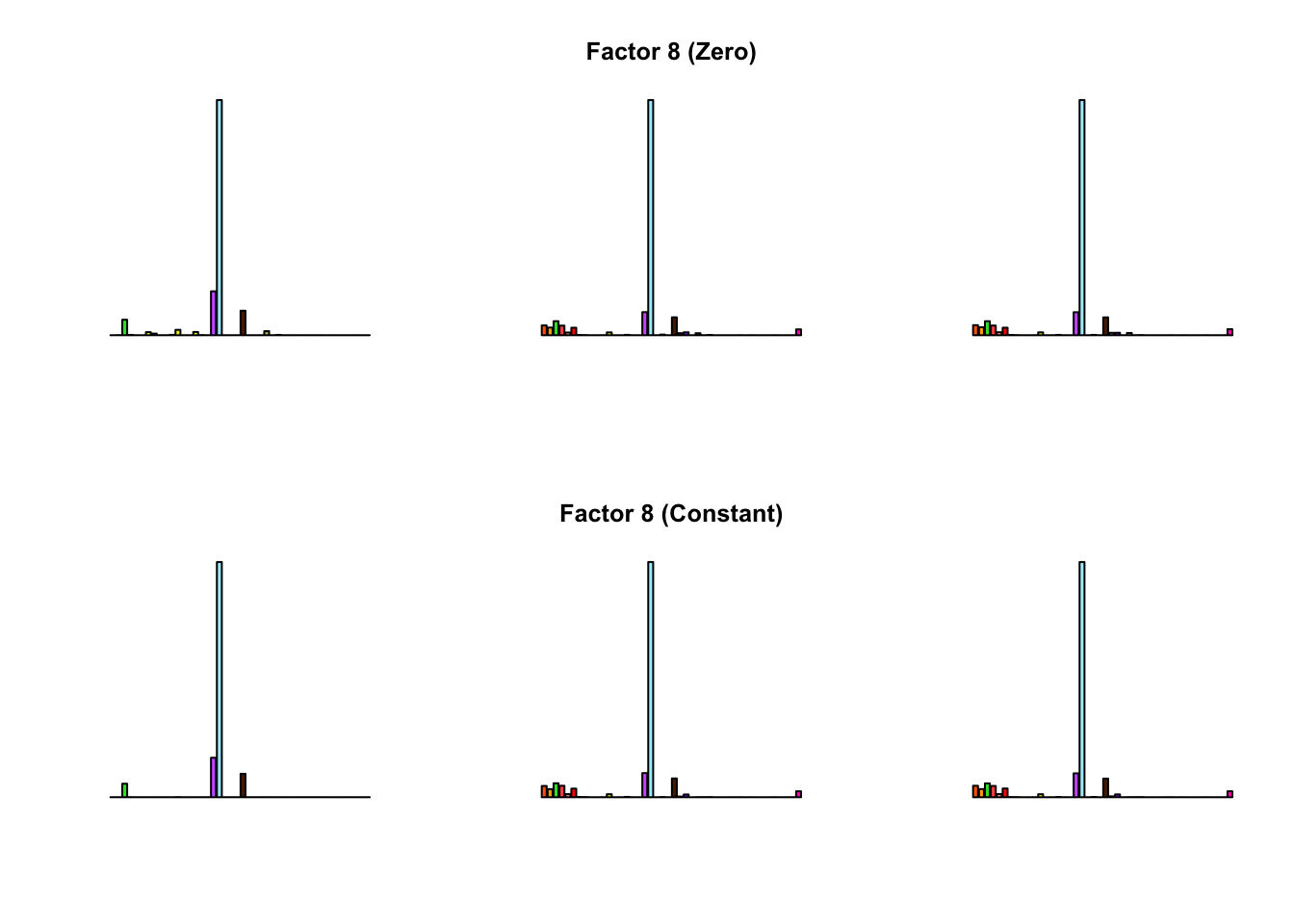
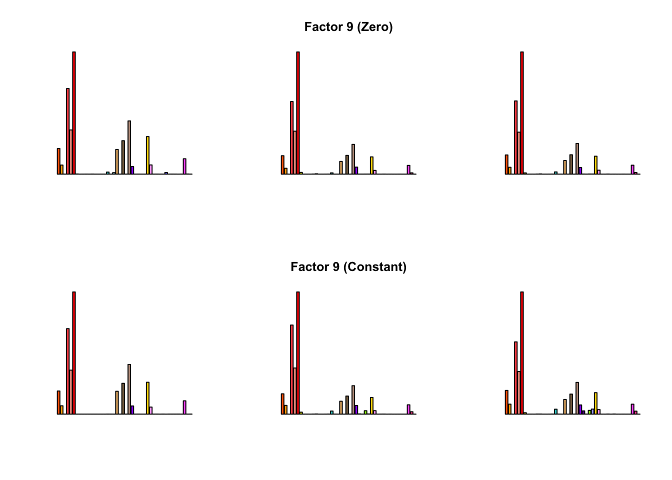
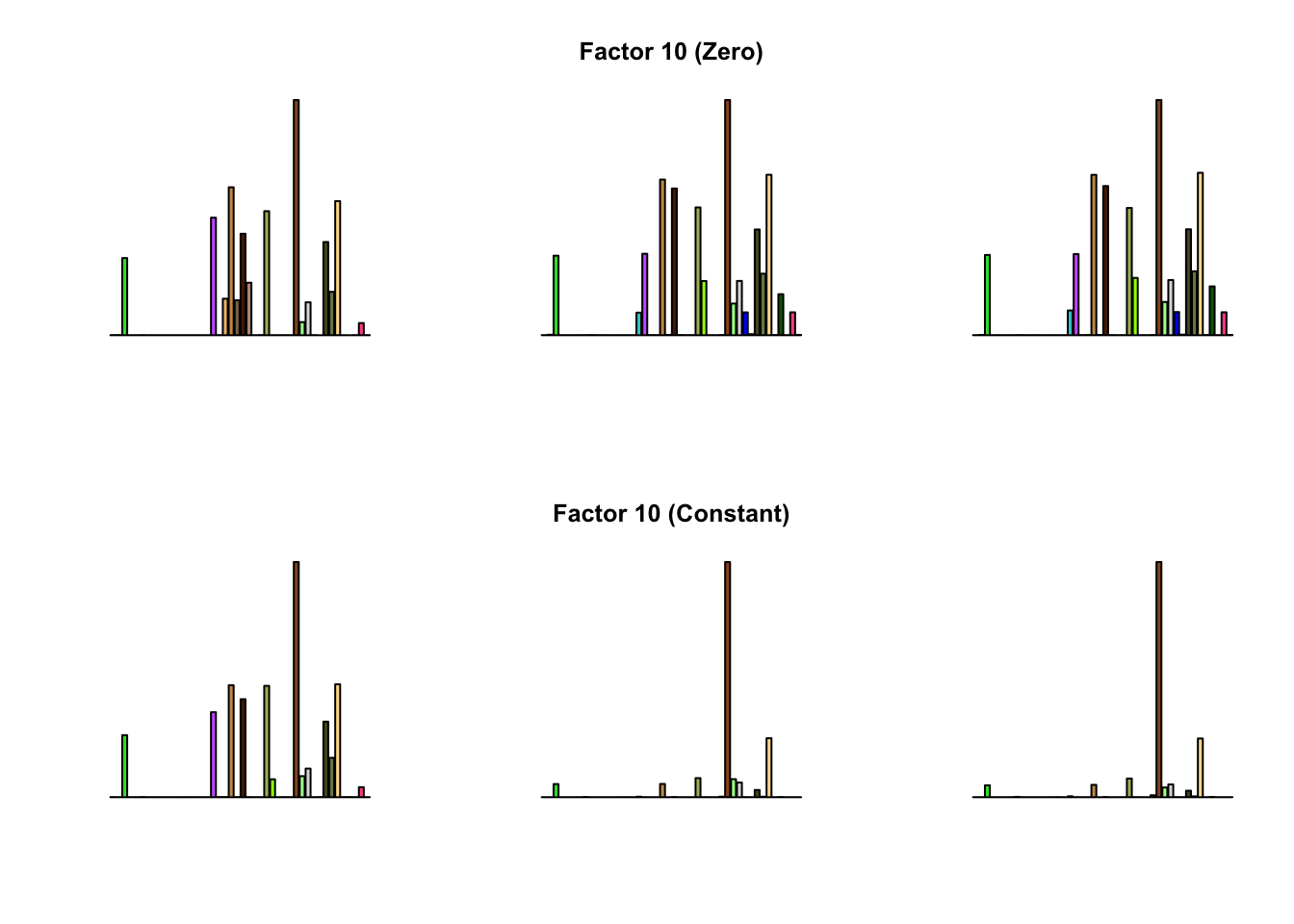
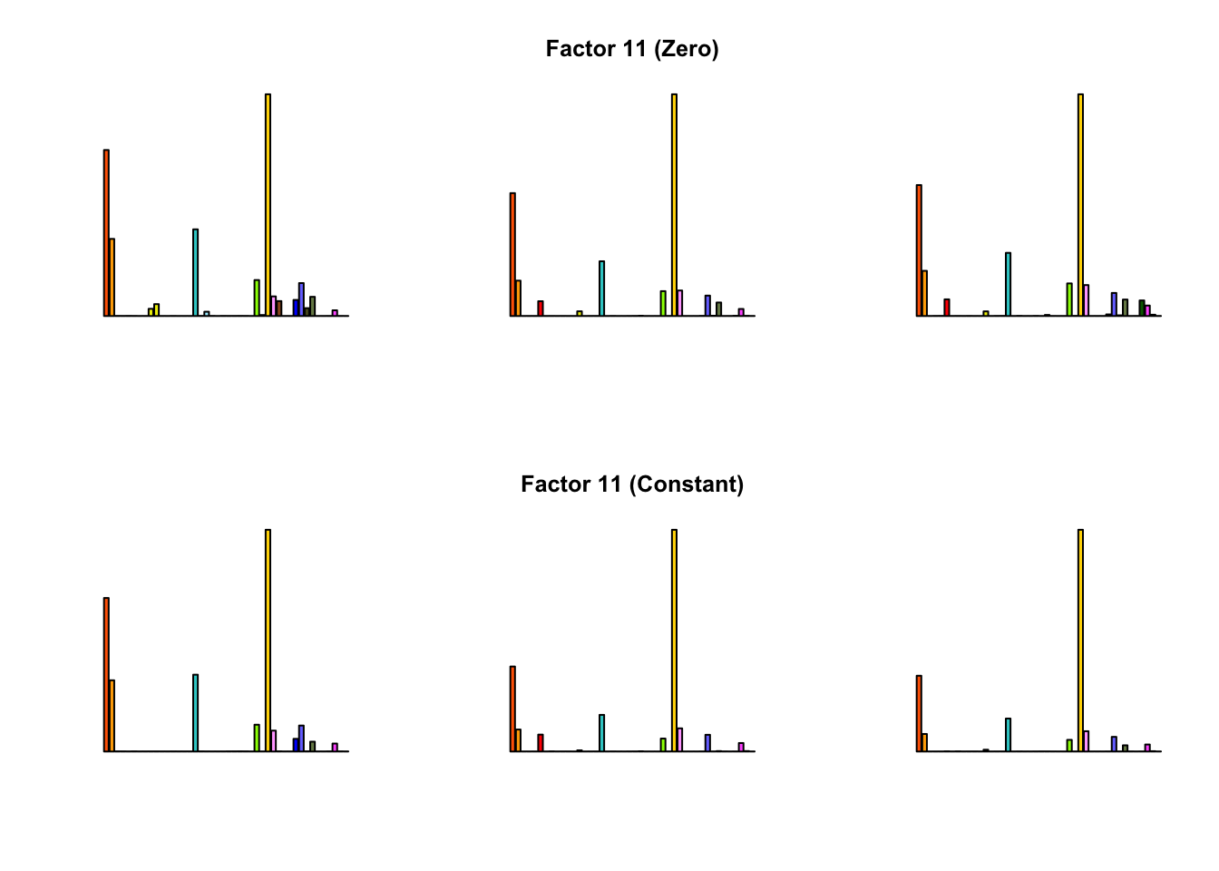
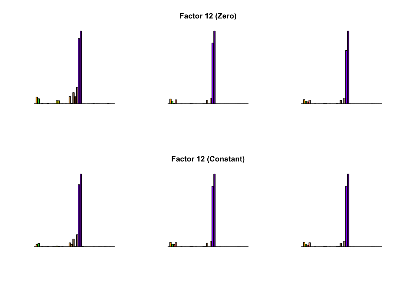
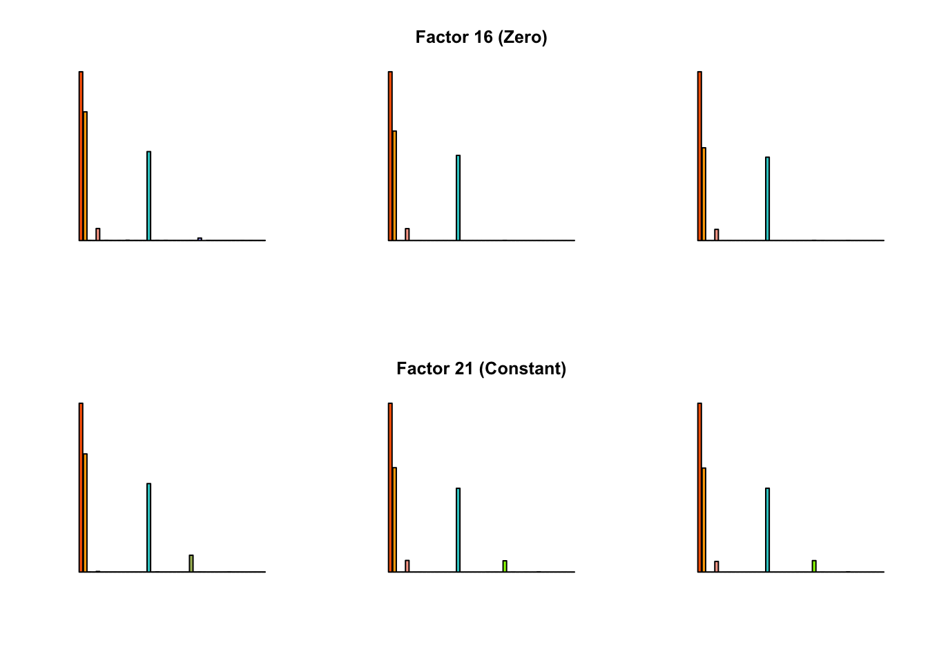
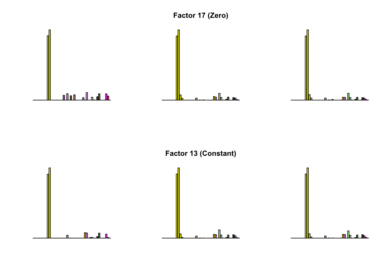
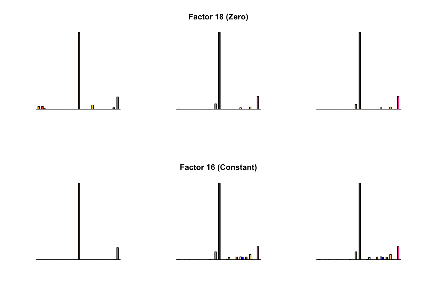
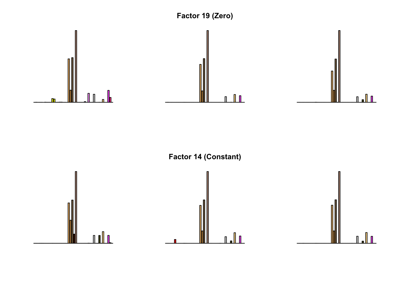
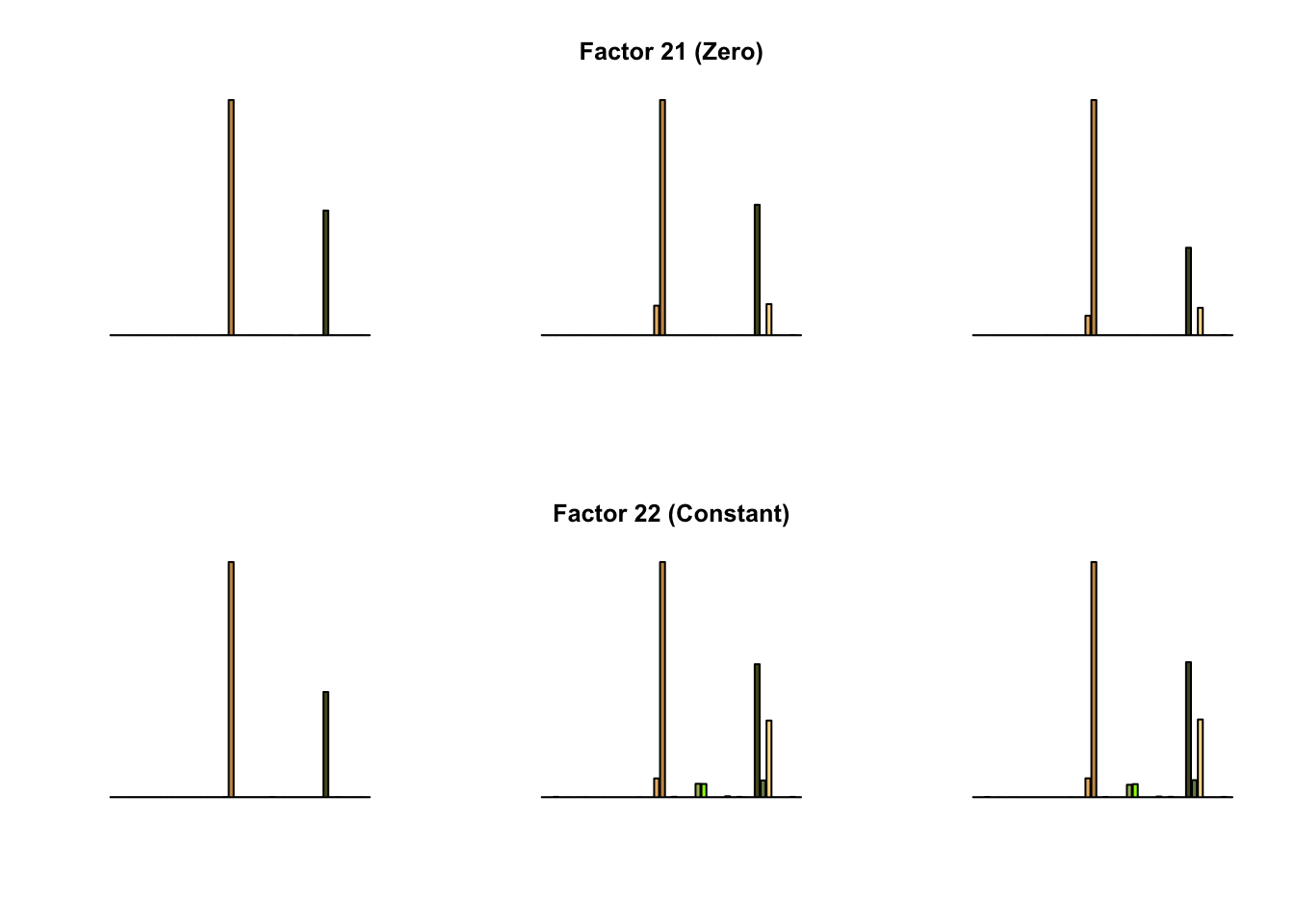
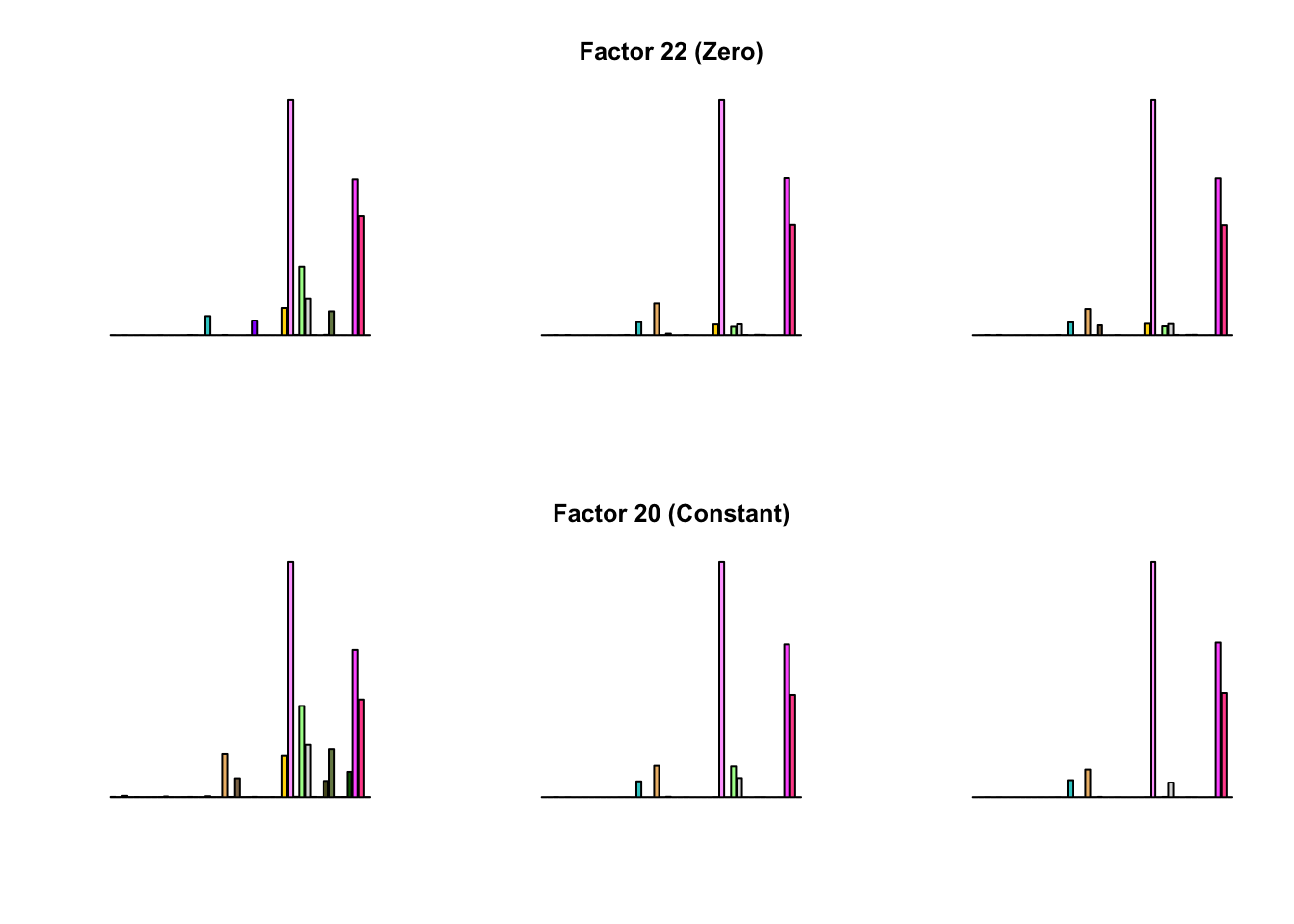
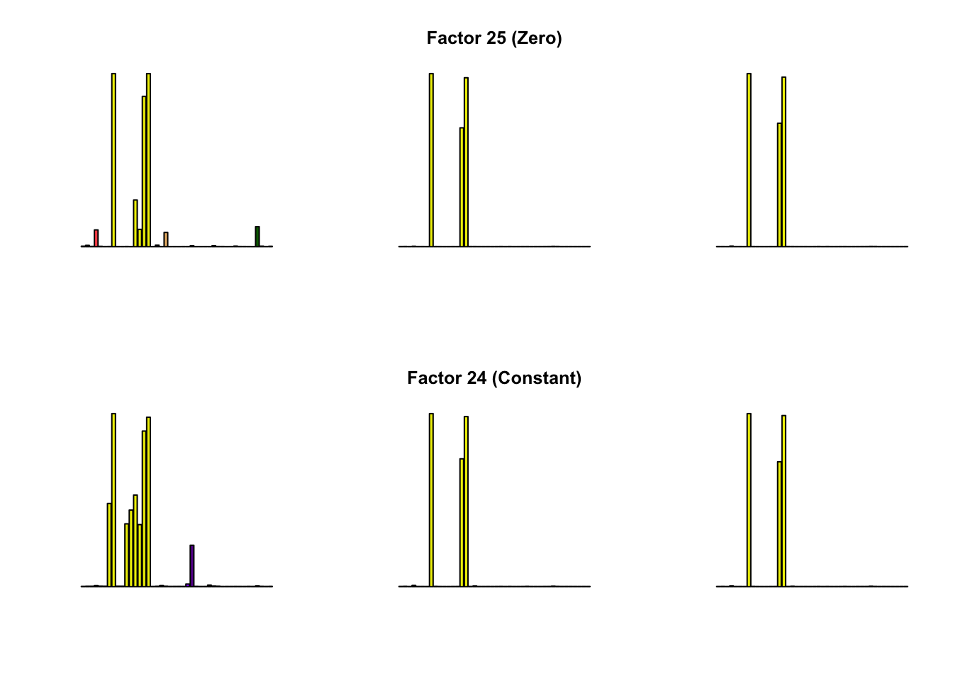
Most of the factors that appear in the “zero” fits but not the “constant” ones correspond to unique effects (which are added as canonical structures anyway). There is one exception, but I’m not sure it’s an important one since it seems to describe correlations that are already captured by Factors 4 and (to a lesser extent) 3:
par(mfrow = c(2, 3))
barplot(fl_g_zero$ldf$f[, 28], col=gtex.colors,
        names.arg = FALSE, axes = FALSE)
barplot(fl_b_zero$ldf$f[, 28], col=gtex.colors,
        names.arg = FALSE, axes = FALSE,
        main = paste("Factor 28 (Zero)"))
barplot(fl_b2_zero$ldf$f[, 28], col=gtex.colors,
        names.arg = FALSE, axes = FALSE)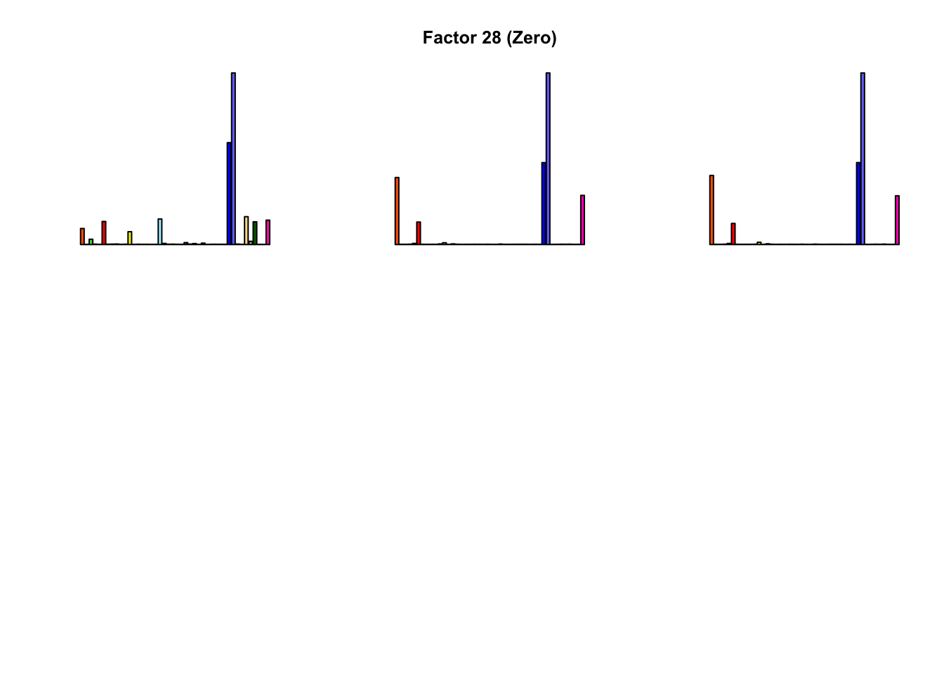
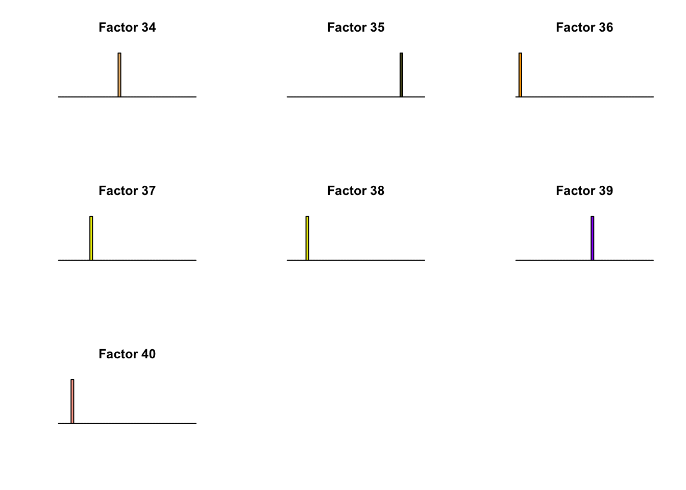
All of the factors found during the second round of fitting (for both variance types) correspond to unique effects. For example, the “zero” variance type adds:
par(mfrow = c(3, 3))
for (k in (fl_b_zero$nfactors + 1):fl_b2_zero$nfactors) {
  barplot(fl_b2_zero$ldf$f[, k], col=gtex.colors,
          names.arg = FALSE, axes = FALSE,
          main = paste("Factor", k))
}
Discussion
Results are very similar, but I think I prefer the “constant” factors. One major difference is in Factor 10, where the “zero” variance structure produces something that is difficult to interpret while the “constant” structure produces a much sparser factor. The other major difference is in Factor 28, but as I argued above, I’m not sure that this factor corresponds to anything real.
I think we can get away with a single round of fitting. For the most part, the factors that are added during the first round change very little, and the new factors are well represented by unique effects (which, as pointed out above) are added as canonical structures anyway.
So, if forced to choose, I’d go with the “constant” variance type and a single round of greedily adding factors and backfitting. This can be done in under 20 minutes on a modern laptop.
A further recommendation would be to prune the results before converting the factors to covariance matrices. That is, I don’t see any need to pass along the factors that are well-represented by unique effects. Something like the following function would do the trick (click “Code” to expand):
# Only keep factors with at least two values greater than 1 / sqrt(n)
find_nonunique_effects <- function(fl) {
  thresh <- 1/sqrt(ncol(fl$fitted_values))
  vals_above_avg <- colSums(fl$ldf$f > thresh)
  nonuniq_effects <- which(vals_above_avg > 1)
  return(fl$ldf$f[, nonuniq_effects, drop = FALSE])
}
Code
Click “Code” to view the code used to obtain the above results.
devtools::load_all("~/GitHub/flashr/")
devtools::load_all("~/GitHub/ebnm/")

gtex <- readRDS(gzcon(url("https://github.com/stephenslab/gtexresults/blob/master/data/MatrixEQTLSumStats.Portable.Z.rds?raw=TRUE")))
strong <- gtex$strong.z
strong_data <- flash_set_data(strong, S = 1)

my_init_fn <- function(Y, K = 1) {
  ret = udv_si(Y, K)
  pos_sum = sum(ret$v[ret$v > 0])
  neg_sum = -sum(ret$v[ret$v < 0])
  if (neg_sum > pos_sum) {
    return(list(u = -ret$u, d = ret$d, v = -ret$v))
  } else
    return(ret)
}

# Using mixSQP maybe requires try/catch?

ebnm_fn = "ebnm_ash"
ebnm_param = list(l = list(mixcompdist = "normal",
                           optmethod = "mixSQP"),
                  f = list(mixcompdist = "+uniform",
                           optmethod = "mixSQP"))

# var_type = "zero" -----------------------------------------------------

t_g_zero <- system.time(
  fl_g_zero <- flashr:::flash_greedy_workhorse(strong_data,
                                               var_type = "zero",
                                               ebnm_fn = ebnm_fn,
                                               ebnm_param = ebnm_param,
                                               init_fn = "my_init_fn",
                                               stopping_rule = "factors",
                                               tol = 1e-3,
                                               verbose_output = "odF")
) # 34 factors in 5.5 min
saveRDS(fl_g_zero, "~/GitHub/MASHvFLASH/output/MASHvFLASHnn2/fl_g_zero.rds")
saveRDS(t_g_zero, "~/GitHub/MASHvFLASH/output/MASHvFLASHnn2/t_g_zero.rds")

t_b_zero <- system.time(
  fl_b_zero <- flashr::flash_backfit_workhorse(strong_data,
                                               f_init = fl_g_zero,
                                               var_type = "zero",
                                               ebnm_fn = ebnm_fn,
                                               ebnm_param = ebnm_param,
                                               stopping_rule = "factors",
                                               tol = 1e-3,
                                               verbose_output = "odF")
) # backfit in 15.0 minutes
saveRDS(fl_b_zero, "~/GitHub/MASHvFLASH/output/MASHvFLASHnn2/fl_b_zero.rds")
saveRDS(t_b_zero, "~/GitHub/MASHvFLASH/output/MASHvFLASHnn2/t_b_zero.rds")

t_g2_zero <- system.time(
  fl_g2_zero <- flashr:::flash_greedy_workhorse(strong_data,
                                                f_init = fl_b_zero,
                                                var_type = "zero",
                                                ebnm_fn = ebnm_fn,
                                                ebnm_param = ebnm_param,
                                                init_fn = "my_init_fn",
                                                stopping_rule = "factors",
                                                tol = 1e-3,
                                                verbose_output = "odF")
) # 6 more factors in 0.8 min
saveRDS(fl_g2_zero, "~/GitHub/MASHvFLASH/output/MASHvFLASHnn2/fl_g2_zero.rds")
saveRDS(t_g2_zero, "~/GitHub/MASHvFLASH/output/MASHvFLASHnn2/t_g2_zero.rds")

t_b2_zero <- system.time(
  fl_b2_zero <- flashr::flash_backfit_workhorse(strong_data,
                                                f_init = fl_g2_zero,
                                                var_type = "zero",
                                                ebnm_fn = ebnm_fn,
                                                ebnm_param = ebnm_param,
                                                stopping_rule = "factors",
                                                tol = 1e-3,
                                                verbose_output = "odF")
) # backfit in 20.7 minutes
saveRDS(fl_b2_zero, "~/GitHub/MASHvFLASH/output/MASHvFLASHnn2/fl_b2_zero.rds")
saveRDS(t_b2_zero, "~/GitHub/MASHvFLASH/output/MASHvFLASHnn2/t_b2_zero.rds")

t_g3_zero <- system.time(
  fl_g3_zero <- flashr:::flash_greedy_workhorse(strong_data,
                                                f_init = fl_b2_zero,
                                                var_type = "zero",
                                                ebnm_fn = ebnm_fn,
                                                ebnm_param = ebnm_param,
                                                init_fn = "my_init_fn",
                                                stopping_rule = "factors",
                                                tol = 1e-3,
                                                verbose_output = "odF")
)
# Nothing added this time!


# var_type = "const" ----------------------------------------------------

t_g_const <- system.time(
  fl_g_const <- flashr:::flash_greedy_workhorse(strong,
                                                var_type = "constant",
                                                ebnm_fn = ebnm_fn,
                                                ebnm_param = ebnm_param,
                                                init_fn = "my_init_fn",
                                                stopping_rule = "factors",
                                                tol = 1e-3,
                                                verbose_output = "odF")
) # 26 factors in 3.3 min
saveRDS(fl_g_const, "~/GitHub/MASHvFLASH/output/MASHvFLASHnn2/fl_g_const.rds")
saveRDS(t_g_const, "~/GitHub/MASHvFLASH/output/MASHvFLASHnn2/t_g_const.rds")

t_b_const <- system.time(
  fl_b_const <- flashr::flash_backfit_workhorse(strong,
                                                f_init = fl_g_const,
                                                var_type = "constant",
                                                ebnm_fn = ebnm_fn,
                                                ebnm_param = ebnm_param,
                                                stopping_rule = "factors",
                                                tol = 1e-3,
                                                verbose_output = "odF")
) # backfit in 13.1 min
saveRDS(fl_b_const, "~/GitHub/MASHvFLASH/output/MASHvFLASHnn2/fl_b_const.rds")
saveRDS(t_b_const, "~/GitHub/MASHvFLASH/output/MASHvFLASHnn2/t_b_const.rds")

t_g2_const <- system.time(
  fl_g2_const <- flashr:::flash_greedy_workhorse(strong,
                                                 f_init = fl_b_const,
                                                 var_type = "constant",
                                                 ebnm_fn = ebnm_fn,
                                                 ebnm_param = ebnm_param,
                                                 init_fn = "my_init_fn",
                                                 stopping_rule = "factors",
                                                 tol = 1e-3,
                                                 verbose_output = "odF")
) # 2 more factors in 0.4 min
saveRDS(fl_g2_const, "~/GitHub/MASHvFLASH/output/MASHvFLASHnn2/fl_g2_const.rds")
saveRDS(t_g2_const, "~/GitHub/MASHvFLASH/output/MASHvFLASHnn2/t_g2_const.rds")

t_b2_const <- system.time(
  fl_b2_const <- flashr::flash_backfit_workhorse(strong,
                                                 f_init = fl_g2_const,
                                                 var_type = "constant",
                                                 ebnm_fn = ebnm_fn,
                                                 ebnm_param = ebnm_param,
                                                 stopping_rule = "factors",
                                                 tol = 1e-3,
                                                 verbose_output = "odF")
) # backfit in 9.4 min
saveRDS(fl_b2_const, "~/GitHub/MASHvFLASH/output/MASHvFLASHnn2/fl_b2_const.rds")
saveRDS(t_b2_const, "~/GitHub/MASHvFLASH/output/MASHvFLASHnn2/t_b2_const.rds")

t_g3_const <- system.time(
  fl_g3_const <- flashr:::flash_greedy_workhorse(strong,
                                                 f_init = fl_b2_const,
                                                 var_type = "constant",
                                                 ebnm_fn = ebnm_fn,
                                                 ebnm_param = ebnm_param,
                                                 init_fn = "my_init_fn",
                                                 stopping_rule = "factors",
                                                 tol = 1e-3,
                                                 verbose_output = "odF")
)
# Nothing new added.
Session information
sessionInfo()R version 3.4.3 (2017-11-30)
Platform: x86_64-apple-darwin15.6.0 (64-bit)
Running under: macOS High Sierra 10.13.6
Matrix products: default
BLAS: /Library/Frameworks/R.framework/Versions/3.4/Resources/lib/libRblas.0.dylib
LAPACK: /Library/Frameworks/R.framework/Versions/3.4/Resources/lib/libRlapack.dylib
locale:
[1] en_US.UTF-8/en_US.UTF-8/en_US.UTF-8/C/en_US.UTF-8/en_US.UTF-8
attached base packages:
[1] stats graphics grDevices utils datasets methods base
loaded via a namespace (and not attached):
[1] workflowr_1.0.1 Rcpp_0.12.18 digest_0.6.15
[4] rprojroot_1.3-2 R.methodsS3_1.7.1 backports_1.1.2
[7] git2r_0.21.0 magrittr_1.5 evaluate_0.10.1
[10] stringi_1.1.6 whisker_0.3-2 R.oo_1.21.0
[13] R.utils_2.6.0 rmarkdown_1.8 tools_3.4.3
[16] stringr_1.3.0 yaml_2.1.17 compiler_3.4.3
[19] htmltools_0.3.6 knitr_1.20 This reproducible R Markdown analysis was created with workflowr 1.0.1