Parallel backfits
Jason Willwerscheid
7/6/2019
Last updated: 2019-07-10
Checks: 6 0
Knit directory: FLASHvestigations/
This reproducible R Markdown analysis was created with workflowr (version 1.2.0). The Report tab describes the reproducibility checks that were applied when the results were created. The Past versions tab lists the development history.
Great! Since the R Markdown file has been committed to the Git repository, you know the exact version of the code that produced these results.
Great job! The global environment was empty. Objects defined in the global environment can affect the analysis in your R Markdown file in unknown ways. For reproduciblity it’s best to always run the code in an empty environment.
The command set.seed(20180714) was run prior to running the code in the R Markdown file. Setting a seed ensures that any results that rely on randomness, e.g. subsampling or permutations, are reproducible.
Great job! Recording the operating system, R version, and package versions is critical for reproducibility.
Nice! There were no cached chunks for this analysis, so you can be confident that you successfully produced the results during this run.
Great! You are using Git for version control. Tracking code development and connecting the code version to the results is critical for reproducibility. The version displayed above was the version of the Git repository at the time these results were generated.
Note that you need to be careful to ensure that all relevant files for the analysis have been committed to Git prior to generating the results (you can use wflow_publish or wflow_git_commit). workflowr only checks the R Markdown file, but you know if there are other scripts or data files that it depends on. Below is the status of the Git repository when the results were generated:
Ignored files:
    Ignored:    .DS_Store
    Ignored:    .Rhistory
    Ignored:    .Rproj.user/
    Ignored:    analysis/.DS_Store
    Ignored:    code/.DS_Store
    Ignored:    code/flashier_bench/.DS_Store
    Ignored:    data/flashier_bench/

Untracked files:
    Untracked:  code/ebspca.R
Note that any generated files, e.g. HTML, png, CSS, etc., are not included in this status report because it is ok for generated content to have uncommitted changes.
These are the previous versions of the R Markdown and HTML files. If you’ve configured a remote Git repository (see ?wflow_git_remote), click on the hyperlinks in the table below to view them.
| File | Version | Author | Date | Message |
|---|---|---|---|---|
| Rmd | bc8f534 | Jason Willwerscheid | 2019-07-10 | wflow_publish(“analysis/parallel_v2.Rmd”) |
| html | f9a3167 | Jason Willwerscheid | 2019-07-08 | Build site. |
| Rmd | 239862c | Jason Willwerscheid | 2019-07-08 | wflow_publish(c(“analysis/parallel_v2.Rmd”, “analysis/index.Rmd”)) |
| html | 136ecb9 | Jason Willwerscheid | 2019-07-08 | Build site. |
| Rmd | 9cfd41c | Jason Willwerscheid | 2019-07-08 | wflow_publish(“analysis/parallel_v2.Rmd”) |
Introduction
I’ve rewritten flashier’s parallel backfitting algorithm. As before, factors can be backfit in parallel by setting parameter backfit.order = "parallel". The number of cores and type of cluster (socket or fork) can be set using global options (here, I use options(cl.type = "FORK", cl.cores = parallel::detectCores())).
Each worker is responsible for \(\frac{K}{\text{n.cores}}\) calls to ebnm (where \(K\) is the total number of factors), so we can only really expect performance benefits from parallelization when each call to ebnm is fairly computationally intensive and when \(K\) is somewhat large. Further, since parallel updates are not guaranteed to produce a monotonic increase in the objective function, serial updates should generally be preferred when the dataset is not large.
Test Cases
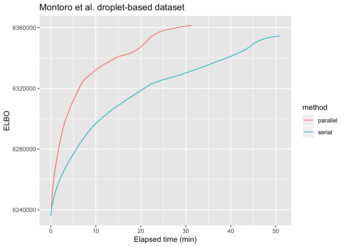
For large problems, parallelization can provide a noticeable speedup. As a first test case, I greedily fit 50 factors to the droplet-based 3’ scRNA-seq dataset from Montoro et al., which is, I think, on the smaller end of the scale of dataset that could benefit from parallel backfitting updates. The dataset, which I also used to benchmark flashier, is described here. I backfit using both the default serial method and the new implementation of the parallel approach. As shown below, parallel updates are able to attain the same ELBO as the serial method about three times more quickly.
library(ggplot2)

timing <- readRDS("./output/parallel_v2/sp_trachea_timing.rds")

serial.res <- data.table::fread("./output/parallel_v2/sp_trachea_serial.txt")
serial.res$method <- "serial"
serial.res$time <- timing$serial * 1:nrow(serial.res) / nrow(serial.res)

parallel.res <- data.table::fread("./output/parallel_v2/sp_trachea_parallel.txt")
parallel.res$method <- "parallel"
parallel.res$time <- timing$parallel * 1:nrow(parallel.res) / nrow(parallel.res)

all.res <- rbind(serial.res, parallel.res)
all.res$time <- as.numeric(all.res$time)

ggplot(all.res, aes(x = time, y = Obj, color = method)) + geom_line() +
  labs(x = "Elapsed time (min)", y = "ELBO", title = "Montoro et al. droplet-based dataset")
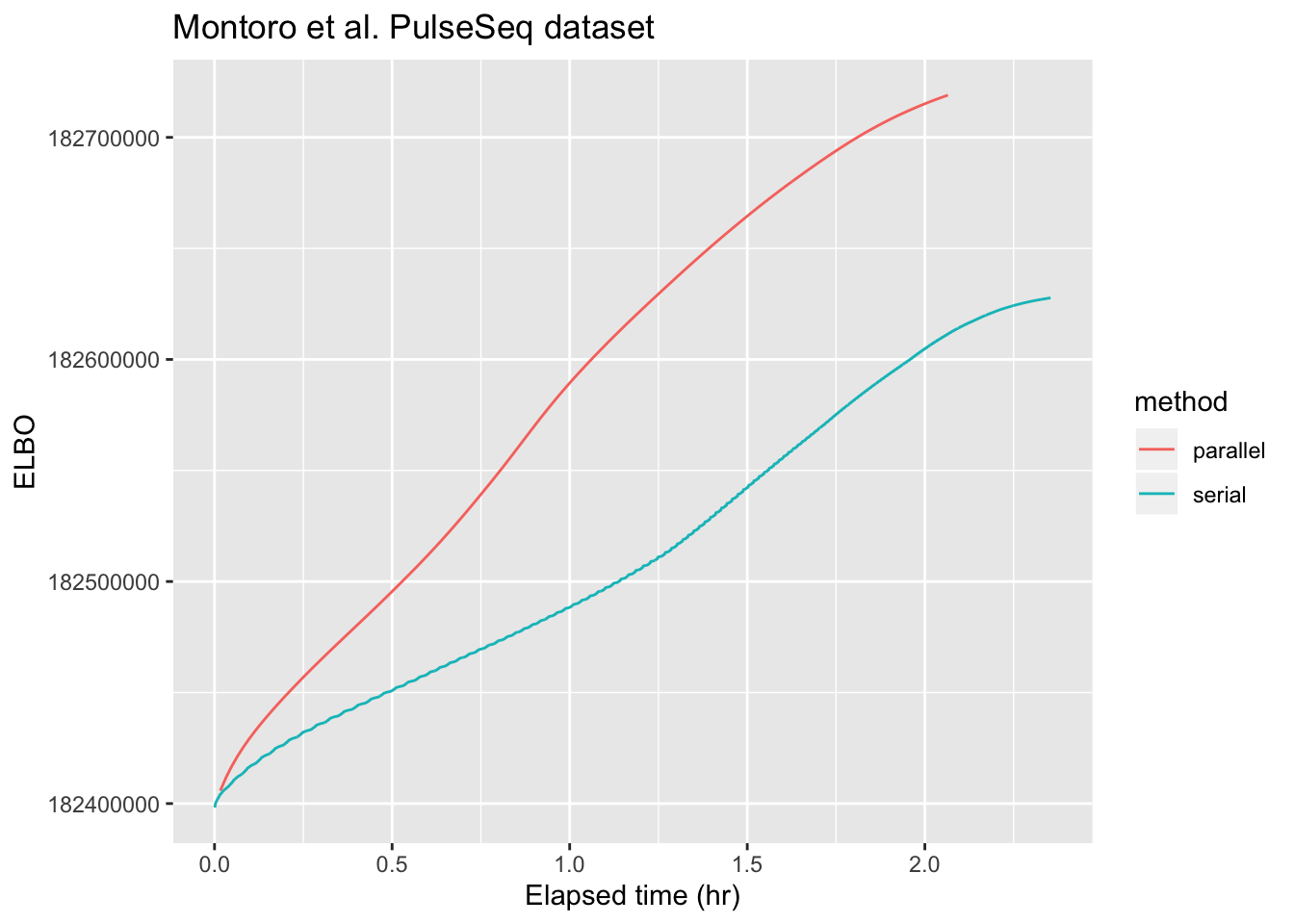
Next, I repeat the experiment on the larger PulseSeq dataset from Montoro et al. (described here). I get bus errors when I try to use all available cores (using parallel::detectCores()), so I lower cl.cores to 16. (For both of these datasets, however, there is not much additional speedup after the first 8 cores.) Here, parallel updates are only about twice as fast as serial ones.
Do note, however, that the default backfitting method already uses some tricks to speed up backfits. In particular, it stops updating any given factor when that factor appears to have converged. For example, factor 42 only gets updated 10 times, while factor 6 must be updated 249 times before it is considered to have converged. As a result, any changes that occur in the final 239 backfitting iterations will not be reflected in the final form of factor 42. In contrast, parallel backfits update every factor every time, so with the tolerance parameter set appropriately, parallel backfits will get one close to a local maximum much more reliably. It’s possible to get the same reliability with serial backfits by setting backfit.order = "sequential", but this will be much slower than the default method.
library(ggplot2)

timing <- readRDS("./output/parallel_v2/pulseseq_timing.rds")

serial.res <- data.table::fread("./output/parallel_v2/pulseseq_serial.txt")
serial.res$method <- "serial"
serial.res$time <- timing$serial * 1:nrow(serial.res) / nrow(serial.res)

parallel.res <- data.table::fread("./output/parallel_v2/pulseseq_parallel.txt")
parallel.res$method <- "parallel"
parallel.res$time <- timing$parallel * 1:nrow(parallel.res) / nrow(parallel.res)

all.res <- rbind(serial.res, parallel.res)
all.res$time <- as.numeric(all.res$time)

ggplot(all.res, aes(x = time, y = Obj, color = method)) + geom_line() +
  labs(x = "Elapsed time (hr)", y = "ELBO", title = "Montoro et al. PulseSeq dataset")
Limitations
Variance Structure
For now, I’ve restricted parallel backfits to the case where residual variance is assumed to be constant across all entries (var.type = 0). Whereas sequential backfitting can take advantage of the fact that the update to expected residuals is rank-one, parallel backfits must re-estimate the residual variance from scratch at each iteration. Recall that the most useful variance structures (row-wise, column-wise, and constant) can be estimated as simple functions of expected squared residuals (row-wise means, column-wise means, and the overall mean). Recall also that flashier doesn’t usually store a full matrix of residuals \(R\), so that the expected squared residual \(R_{ij}^2\) must be calculated as:
\[ \mathbb{E} R_{ij}^2 = \mathbb{E} (Y_{ij} - \sum_k L_{ik} F_{jk})^2 = Y_{ij}^2 - 2 Y_{ij} \sum_k \mathbb{E} L_{ik} \mathbb{E} F_{jk} + \sum_{k \ne \ell} \mathbb{E} L_{ik} \mathbb{E} F_{jk} \mathbb{E} L_{i\ell} \mathbb{E} F_{j\ell} + \sum_k \mathbb{E} L_{ik}^2 \mathbb{E} F_{jk}^2 \]
When residual variance is constant across all entries, we only need \(\sum_{i, j} R_{ij}^2\), and each of the above terms can be efficiently summed over \(i\) and \(j\). The trick, of course, is to move the summation over \(i\) and \(j\) to the inside (and to pre-compute \(\sum_{i, j} Y_{ij}^2\)). For example,
\[ \sum_{i, j} \sum_{k \ne \ell} \mathbb{E} L_{ik} \mathbb{E} F_{jk} \mathbb{E} L_{i\ell} \mathbb{E} F_{j\ell} = \sum_{k, \ell} \sum_i \mathbb{E} L_{ik} \mathbb{E} L_{i\ell} \sum_j \mathbb{E} F_{jk} \mathbb{E} F_{j\ell} - \sum_k \sum_i (\mathbb{E} L_{ik})^2 \sum_j (\mathbb{E} F_{jk})^2 \]
The first term on the RHS can be computed as sum(crossprod(EL) * crossprod(EF)); the second can be computed as sum(colSums(EL^2) * colSums(EF^2)).
For row-wise or column-wise variance structures, however, the first term is much more difficult to compute. Instead of simply taking crossproducts, one must form a \(n \times k^2\) (or \(p \times k^2\)) matrix, so that unless \(k^2 \ll n\) (or \(k^2 \ll p\)), one would not be much worse off by simply storing the matrix of expected residuals. But we only stand to benefit from parallelization when we are doing large backfits on large data matrices; that is, when \(k\) is not small and when storing a matrix of residuals is expensive.
Fixed factors
I haven’t implemented parallel updates for fixed factors, mainly because the handling is more complicated, but also because parallel updates can run into trouble when factor loadings are not approximately orthogonal. Consider, as an illustration, the case where loadings on two factors are identical. Then loadings updates will also be identical, and the updates to the expected residuals will be double what it would be if the factors were updated one at a time. This kind of situation can easily spiral out of control, as detailed in this example.
Code
The code used in this analysis can be viewed here. TheR package versions used are those that appear in the session information below (“other attached packages”).
sessionInfo()#> R version 3.5.3 (2019-03-11)
#> Platform: x86_64-apple-darwin15.6.0 (64-bit)
#> Running under: macOS Mojave 10.14.5
#>
#> Matrix products: default
#> BLAS: /Library/Frameworks/R.framework/Versions/3.5/Resources/lib/libRblas.0.dylib
#> LAPACK: /Library/Frameworks/R.framework/Versions/3.5/Resources/lib/libRlapack.dylib
#>
#> locale:
#> [1] en_US.UTF-8/en_US.UTF-8/en_US.UTF-8/C/en_US.UTF-8/en_US.UTF-8
#>
#> attached base packages:
#> [1] stats graphics grDevices utils datasets methods base
#>
#> other attached packages:
#> [1] ggplot2_3.2.0 mixsqp_0.1-119 ashr_2.2-38 ebnm_0.1-24
#> [5] flashier_0.1.7
#>
#> loaded via a namespace (and not attached):
#> [1] Rcpp_1.0.1 pillar_1.3.1 compiler_3.5.3
#> [4] git2r_0.25.2 workflowr_1.2.0 iterators_1.0.10
#> [7] tools_3.5.3 digest_0.6.18 tibble_2.1.1
#> [10] evaluate_0.13 gtable_0.3.0 lattice_0.20-38
#> [13] pkgconfig_2.0.2 rlang_0.3.1 Matrix_1.2-15
#> [16] foreach_1.4.4 yaml_2.2.0 parallel_3.5.3
#> [19] xfun_0.6 withr_2.1.2 dplyr_0.8.0.1
#> [22] stringr_1.4.0 knitr_1.22 fs_1.2.7
#> [25] tidyselect_0.2.5 rprojroot_1.3-2 grid_3.5.3
#> [28] data.table_1.12.2 glue_1.3.1 R6_2.4.0
#> [31] rmarkdown_1.12 purrr_0.3.2 magrittr_1.5
#> [34] whisker_0.3-2 backports_1.1.3 scales_1.0.0
#> [37] codetools_0.2-16 htmltools_0.3.6 MASS_7.3-51.1
#> [40] assertthat_0.2.1 colorspace_1.4-1 labeling_0.3
#> [43] stringi_1.4.3 lazyeval_0.2.2 doParallel_1.0.14
#> [46] pscl_1.5.2 munsell_0.5.0 truncnorm_1.0-8
#> [49] SQUAREM_2017.10-1 crayon_1.3.4